Numerical modelling of three dimensional thermal surface discharges

Full text

(1)Engineering Applications of Computational Fluid Mechanics Vol. 5, No. 2, pp. 201–209 (2011). NUMERICAL MODELLING OF THREE-DIMENSIONAL THERMAL SURFACE DISCHARGES Jafar Ali*, John Fieldhouse and Chris Talbot University of Huddersfield, Queensgate, Huddersfield, HD1 3DH, United Kingdom * E-Mail: j.ali@hud.ac.uk (Corresponding Author) ABSTRACT: The use of canal water for cooling is an important opportunity for companies to reduce their carbon emissions and save on energy bills. The available models used to evaluate the possibility of using canal water are too complicated and their applications are difficult. As such some potential opportunities for using canal water for cooling are being lost. This paper addresses current concerns to produce an interactive numerical model that will produce a three dimensional representation of the temperature distribution of heated water discharged into a still water region. The interactive model may be manipulated by non technical personnel to evaluate different discharge scenarios and ensure that the proposal does not infringe the stringent regulations imposed by the Environmental Agencies. The proposed model makes use of information gathered from real on-site testing using a thermal camera and grid measurements in addition to a laboratory experimental tank that duplicates the various on-site options. The parameters of temperature, velocity and boundaries were determined in both practical processes using a predefined grid mesh that covered the mixing zone. These practical results gave the turbulent diffusivity which was then used in the formulation of the model that was optimised to represent the real system results. It is shown that the results from the on-site testing, the laboratory results and the 3-D model all give complementary values so validating the final model. Keywords:. thermal discharge, thermal pollution, turbulent heat diffusion. horizontally into the surface of shallow and still receiving canal water. The thermal discharge studies are classified into three categories, namely theoretical analysis, computational analysis and experimental work. In this paper the experimental and theoretical analyses were undertaken to investigate the behaviour of the thermal discharge plume. Enormous literatures of thermal discharge studies are available; all aiming to minimize the impact of the thermal discharge by reducing its temperature before entering the receiving water. Abramovich (1963) mentioned that the first attempt of computing the jet trajectory in cross flow was made by Baturin and Shepelev in 1934. They obtained the velocity along the centreline of the jet geometrically using velocity vector for the ambient and the jet. The mathematical modelling of three dimensional heated surface jets by McGuirk and Rodi (1978) is a broad study carried out in the late seventies on discharge heated water into stagnant and deep water. The paper solved the five governing equations: continuity equation, two momentum equations in x, y directions, thermal energy equation and the equation of state. The authors made several assumptions to simplify the elliptic equations to parabolic form to. 1. INTRODUCTION The current architectural trend is to build large complexes and manage them centrally. Numerous commercial organisations occupy small spaces in large office blocks where computing facilities are common – all generating heat. To control overall building temperatures it is a necessity to include a cooling system in the building plans at the outset. Traditional air conditioning makes use of chillers to cool the system, but if the building is located in close proximity to a water source then an environmentally friendly alternative may be available. After water has been used for cooling it is returned to the canal in a heated state as a thermal plume emerging from the end of a pipe, see Fig. 1. It is the boundaries of the plume that must be predicted with reasonable accuracy so that environmental legislation is not infringed and riparian ecology is not jeopardised. This study is aimed at addressing that situation to provide a valid interactive 3-dimensional model that will better evaluate the potential of using water sources for cooling purposes and to prevent the circulation of heated discharge into the cooling water intake. The model predicts heat diffusion profile of thermal plume discharging. Received: 15 Aug. 2010; Revised: 10 Dec. 2010; Accepted: 15 Dec. 2010 201.

(2) Engineering Applications of Computational Fluid Mechanics Vol. 5, No. 2 (2010). Thermal plume. x, U, Dx. y, V, Dy. Fig. 1. Thermal plume.. Fig. 2. Central Service Building site at University of Huddersfield.. temperature dilution of the thermal jet. Abdalla et al. (2009) investigated recently the structure of a buoyant plume above a point heat source in a ventilated enclosure. They used large-eddy simulation (LES) in their study as well as CFD package Ansys CFX. Despite the good presentation of the model and the obtained results, it cannot be applied to the thermal plume discharging horizontally into shallow and still receiving water. The objective of this paper is to determine the temperature distribution of cooling water discharge into shallow and still receiving water which has not been discussed fully in the past. One of the British Waterways canal sites is selected for experimental analysis as a source of shallow and still receiving water. The site is simulated with a model tank in laboratory; in both cases temperature and velocity were measured at different layers within the mixing region.. simplify the momentum equations. It is assumed that because the flow extends much further in the longitudinal and lateral directions than in the vertical, gradients in the latter are much larger than in the former two, as a consequence turbulent transport is important only in the vertical direction. Accordingly the turbulent momentum and heat fluxes in the longitudinal and lateral directions have been neglected (McGuirk and Rodi, 1978). Despite the broad analysis in this study the model is limited to applications to warm water discharge into surface of deep stagnant water. The study covered a number of previous work carried out in this field till 1978 and commented on the lack of applications and experiments on those works. Horikawa et al. (1979) investigated the discharge heated water in the surface zone using diffusion coefficient. Ozturk et al. (1995) produced a two-dimensional model of thermal discharge into sea using oceanographic density. Qi et al. (2001) modelled a turbulent jet in cross flow, their study focused on the ratio of Reynolds number for the jet and the ambient as well as the momentum flux ratio. Xin (2000) investigated non horizontal multiple jets discharging into shallow flowing receiving water. The study presented a numerical analysis of the jets behaviour. Integral model for turbulent buoyant jets in unbounded stratified flows (Jirka, 2004) is a recent work on thermal submerged discharge. Plume and jet are studied, but still the discharge into shallow and still water has not been discussed fully. Ma et al. (2007) studied the simulation of thermal jets in cross flow. They solved numerically a number of equations namely continuity, momentum and Boussinesq’s hypothesis, to model the jet trajectory and. 2. THEORETICAL ANALYSIS The main equation used to model the temperature distribution of thermal plume is the heat advection diffusion in Eq. (1):. T T T T U V W t x y z  2T  2T  2T  Dx 2  Dy 2  Dz 2 x y z. (1). where T is the mean temperature, t is time, U, V, W are mean velocity components in x, y & z directions respectively and Dx , Dy , Dz are turbulent diffusivities in x, y & z directions respectively. In fact they are summations of 202.

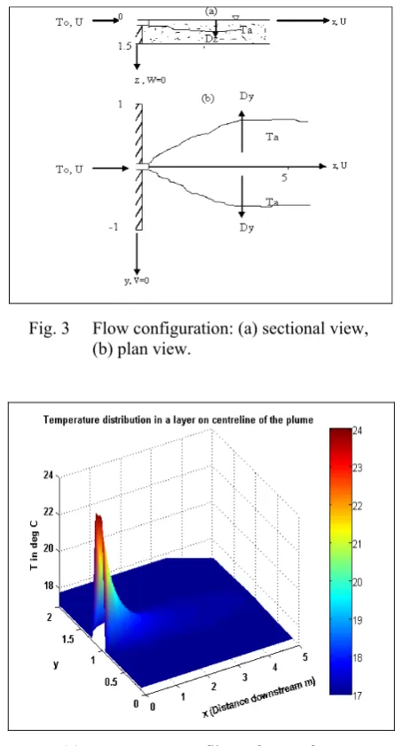
(3) Engineering Applications of Computational Fluid Mechanics Vol. 5, No. 2 (2010). turbulent diffusivity and molecular diffusivity. In this instance the turbulent diffusivity is much greater than the molecular diffusivity value so this is neglected. The canal site considered in this study is shown in Fig. 2. The discharge pipe is horizontal on the surface of canal, so the lateral and vertical velocities V, W are very small and neglected. The longitudinal velocity in x direction is much greater than the diffusivity Dx (Roberts and Webster, 2002) so it is neglected. The advection diffusion equation for steady state flow (no dependence on time) reduces to:. U. T  2T  2T  Dy 2  Dz 2 x y z. (2). Fig. 3. Flow configuration: (a) sectional view, (b) plan view.. Fig. 3 shows a corresponding domain of the flow. The diffusivity values are varied within the turbulence region and from a canal to another depending on the cross section, the depth of the canal, the position of the discharge pipe and so on. The values of D at all grid points are divided by the discharge velocity on the left hand side of Eq. (2):. py  pz . Dy U Dz U. (3) (4). Finite difference method is used to solve the simplified heat advection diffusion Eq. (2) for steady state flow, the result is Eq. (5): (a) Temperature profile on free surface.. T(i 1, j , k )  T( i , j , k ) dx [ p y (T( i , j 1, k )  2T(i , j , k )  T(i , j 1, k ) ) h2  pz (T( i , j ,k 1)  2T( i , j , k )  T(i , j , k 1) )] . (5). where, i, j, k are unit vectors, dx is a strip in x direction and h is a strip in y and z direction, h is equal to the discharge pipe radius. Eq. (5) is able to predict the heat diffusion of the thermal plume at any point and on any layer within the mixing zone. The results obtained from this model give accuracy which is not less than that of previous models. They were mainly focused on solving a number of partial differential equations with significant assumptions to convert the equations from elliptic to parabolic. Fig. 4 illustrate the heat diffusion of the thermal plume on the surface and on a layer below the surface predicted by Eq. (5). The heat diffusion profile presented is for the thermal plume discharged from a single slot into canal, see Fig. 2.. (b) Temperature profile on a layer below free surface. Fig. 4 Temperature distribution from single slot discharge into canal predicted by the numerical model.. 203.

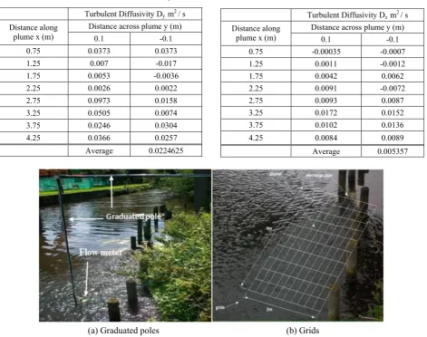
(4) Engineering Applications of Computational Fluid Mechanics Vol. 5, No. 2 (2010). Fig. 5. Coloured multi-diffusers discharge.. Fig. 7. The model also can be applied to determine the heat diffusion profiles in multi diffusers discharge. The thermal plume in Fig. 2 is simulated in the laboratory model tank to three pipes, using the dimensionless densimetric Froude number. Fig. 5 shows dyed heated water discharged from multidiffusers into the tank. Fig. 6 demonstrates the heat diffusion profile for the canal site (Fig. 2) with triple nozzles, Fig. 4a shows the temperature distribution of the plume on the surface of the canal, whilst Fig. 4b shows temperature distribution on a layer below the free surface. The turbulent diffusivity can be determined in several ways; the authors published a paper on the calculation of the turbulent diffusivity in shallow and still water (Ali et al., 2009a). They divided the mixing zone into blocks of elements (Fig. 7) and then the turbulent diffusivity is determined for every individual element. Tables 1 and 2 present the lateral and vertical turbulent diffusivity for a set of elements around the centreline of the plume for the current site. The results indicate some negative values of turbulent diffusivity caused by the transfer of heat from a low heated element to a high heated element due to turbulent eddies. The negative turbulent diffusivity has been investigated theoretically by Avramenko and Basok (2006). Taylor (1921) derived an integral model to predict the diffusion coefficient. He stated that the rate of heat transferred in x direction was determined by the rate of increase of the mean value of the square of the distance, parallel to the axis of x, moved through by a particle of fluid in time t. Wallis and Manson (2004) gathered in a paper all the available methods to predict the diffusion coefficients in thermal discharges.. (a) Temperature profile on free surface.. (b) Temperature profile on a layer below free surface. Fig. 6. Mixing zone divided into elements for diffusivity calculations.. Temperature distribution from multi diffuser discharge into canal predicted by the numerical model.. 204.

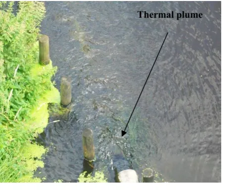
(5) Engineering Applications of Computational Fluid Mechanics Vol. 5, No. 2 (2010). Table 1 Lateral turbulent diffusivity Dy .. Table 2 Vertical turbulent diffusivity Dz .. Turbulent Diffusivity Dy m2 / s Distance along plume x (m). Distance across plume y (m). Distance along plume x (m). 0.1. -0.1. 0.75. 0.0373. 0.0373. 1.25. 0.007. -0.017. 1.75. 0.0053. -0.0036. 2.25. 0.0026. 0.0022. 2.75. 0.0973. 0.0158. 3.25. 0.0505. 0.0074. 3.75. 0.0246. 0.0304. 0.75 1.25 1.75 2.25 2.75 3.25 3.75. 0.0366. 0.0257. 4.25. Average. 0.0224625. 4.25. (a) Graduated poles Fig. 8. -0.00035 0.0011 0.0042 0.0091 0.0093 0.0172 0.0102. -0.0007 -0.0012 0.0062 -0.0072 0.0087 0.0152 0.0136. 0.0084. 0.0089. Average. 0.005357. (b) Grids. Grids and graduated pole holding flow meter and thermocouple.. building cooling system. As such the University is allowed to extract cold water from the canal and discharge warm water into it. To monitor the whole site it was necessary to establish a reference grid over which the results of water flow and temperature would be measured across, along and below the surface of the canal. The centreline of the outlet pipe at its end position served as the origin of the grid. A graduated pole was laid along the bank to give the linear reference points and a second pole was fixed at 90° to the bank to give the transverse reference positions. A third vertical pole was secured to the main pole to which the thermocouple probe and flow meter could be attached. This third pole was also graduated to indicate depth. The arrangement is shown in Fig. 8a and the adopted grids are shown in Fig. 8b. Ambient canal water temperatures were recorded 15m upstream and downstream of the outlet discharge point. Both the ambient canal water and air temperatures were. 3. EXPERIMENTAL PROCEDURE AND EQUIPMENT 3.1. Turbulent Diffusivity Dz m2 / s Distance across plume y (m) 0.1 -0.1. On-site canal. The experiments performed on the actual British Waterways canal sites. These types of experiments give valuable data which cannot be achieved by laboratory work. Since the diffusion is influenced by a number of complicated features, such as the cross section of canal, bed interface, wind effects and so on. They are difficult to be controlled in the laboratory work. In addition the majority of the previous studies were based on experimental laboratory works which have been criticized for the model tank set up. The Central Services Building at University of Huddersfield was selected as the primary site for initial investigations as thermal plume of the flow is clearly defined. This is shown in Figs. 1 and 2. The University has a licence from British Waterways to use the CSB site as part of the 205.

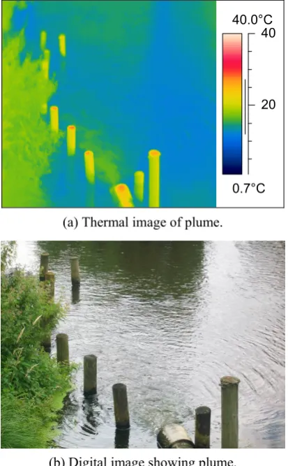
(6) Engineering Applications of Computational Fluid Mechanics Vol. 5, No. 2 (2010). pass. In addition to a single slot discharge, experiments were carried out using multi diffusers with three nozzles, see Fig. 5. The temperatures were measured following the same procedures for the single slot discharge.. recorded at the start and end of the trial run using K type thermocouples with amplifier connected to a data acquisition device, which in turn connected to a laptop. The velocity of the discharge plume was measured by an impeller flow meter. The canal water temperature and velocity were then measured and recorded at the grid points at different depths: the free surface, discharge layer, at mid depth and 50mm above the bed.. 40.0°C 40. 20. 0.7°C. (a) Thermal image of plume.. Fig. 9. 3.2. Dyed hot water discharge into model tank.. Laboratory model tank. The objective of this experiment is to observe the behaviour of the thermal plume in layers below the surface and to model the process under variable conditions such as flow rate, discharge temperature and multi diffusers discharge. The experiment is conducted in a tank, 2m long by 1m wide and 0.3m deep, constructed of acrylic so as to allow visual observation and taking photographs of experiments. The tank is a 1/10th scale model to represent most anticipated situations that may exist in practice. The discharge is supplied from a constant head cistern connected to main hot and cold water pipes with flow control valves to maintain the required temperature, discharge speed is controlled by a valve. A by-pass line was installed to allow preliminary adjustment of temperature and flow before water was discharged into the tank. Coloured hot water discharged into the tank to observe the vertical diffusion of the plume as shown in Fig. 9. Different pipe diameters, temperatures, velocities and locations have been used for the discharge and the effects evaluated. K type thermocouples were used to measure the temperature and the data were transmitted through a data acquisition device (Lab jack 12) to a computer. The water layers below the discharge point is not affected very much by heated water and as a result there will be a path for fishes to. (b) Digital image showing plume. Fig. 10 Thermal and digital images for thermal plume at CSB.. 3.3. Thermal images. Thermal camera is a measurement tool used in the current study to measure the temperature on the surface of mixing zone in canal site and the model tank. Thermal camera shows the temperature distribution on the surface of a hot body by transforming an infrared image coming from a hot body into a coloured image which is representative of the thermal gradients across the body. A typical thermal image and a normal colour image are shown in Fig. 10. The thermal imaging camera was set to a temperature range of 0.7C–40C as shown on the colour bar to the right of the image. In addition to the temperature measurements, the advantage of the thermal images is that it can predict the exact surface area of the mixing zone and the edge of plume in which the survey area will be clearly defined. Temperatures measured by the thermocouples 206.

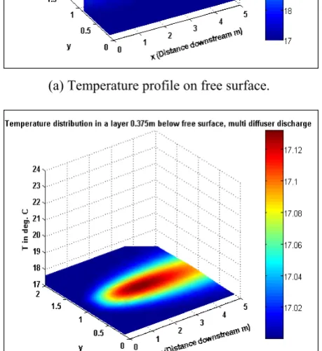
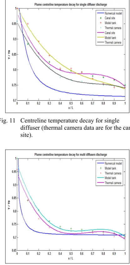
(7) Engineering Applications of Computational Fluid Mechanics Vol. 5, No. 2 (2010). canal site when the discharge pipe is divided to triple nozzles. This test showed the amenability of the model to be extended to multiple discharges. The model in this study is also able to predict the temperature decay along any line within the mixing zone so a complete temperature map may be created of the mixing zone. To examine the accuracy of the theoretical model the temperature along the centreline of the plume (core) was predicted using Eq. (5) and compared with the onsite and laboratory measured data. This predicted centreline temperature of the plume was compared with the associated test values and presented in Figs. 11 & 12. These figures demonstrate the comparison of the results for single and multi-diffuser discharge respectively.. were verified by thermal images data and compared with the model predicted data. The comparison of the results will be presented in the next section. 4. RESULTS DISCUSSION The advection diffusion equation used in this study is an important equation to model diffusion of water and air. The equation does not contain the gravitational effects therefore the derived model will be, in this instance, limited to the surface discharge application. However the turbulent diffusivity is included in the equation so this will to some degree counter concerns regarding the gravitational effects. The finite difference method used to solve the simplified heat diffusion Eq. (2) includes the turbulent diffusivity terms (Dy and Dz ) which were measured empirically (Ali et al., 2009a) on a shallow and still water canal site and applied to the final model. Tables 1 and 2 respectively present the lateral and vertical turbulent diffusivity for the current site study which was the CSB site. Since this was a surface discharge, the results of this model will be applicable to any surface discharge into still and shallow receiving water. The average of the lateral turbulent diffusivity was predicted to be 0.02246 and the vertical turbulent diffusivity predicted to be 0.00536. Accordingly the parameter Py in Eq. (5) will be 0.02246/U and Pz will be 0.00536/U. The discharge velocity U for the current site is 1.23m/s, thus Py = 0.0183 and Pz = 0.0044. The value for strip “dx” for the current site study was selected to be 0.05m (0.005m for the model tank) and the strip “h” equal to the discharge pipe radius. The heat diffusion profile predicted by the final model for CSB site with an initial discharge temperature of 24C and pipe diameter 0.15m is shown in Fig. 4. Fig. 4a shows the temperature distribution on the water surface, whilst Fig. 4b shows the temperature distribution on a layer 0.375m below the surface of the water. In addition to a single discharge, the model can be applied to a multi-diffuser discharges where the overall flow rate is maintained and as such the velocity discharge maintained for each discharge nozzle. A triple discharge was evaluated within the laboratory test rig. The three nozzles were selected to have a total area equal to the single discharge area so the velocities remained the same and the same initial temperature was used for both tests. The heat diffusion profiles for the multidiffuser system are presented in Fig. 6 for CSB. Fig. 11 Centreline temperature decay for single diffuser (thermal camera data are for the canal site).. Fig. 12 Centreline temperature decay for multi diffuser (thermal camera data are for the model tank).. 207.

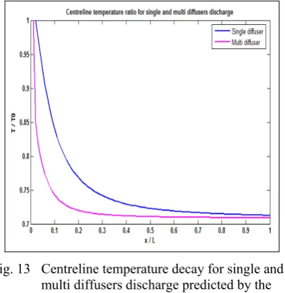
(8) Engineering Applications of Computational Fluid Mechanics Vol. 5, No. 2 (2010). The results for the thermal camera are different from the others because it measures the free surface temperature of the receiving water while the other results are for the discharge layer (this layer is located below the free surface at a depth equal to the radius of the discharge pipe). The temperature decay along the centreline of the plume for the single and multi diffusers discharge are presented in Fig. 13, in this comparison the figure shows similarity for the profiles with an increased rapidly decreasing temperature for the multi-diffuser system.. stages of discharge and then less so further along the plume. . Greater heat diffusion in one direction of discharge will achieve higher turbulent diffusivity in that direction.. NOMENCLATURE T TO t U, V, W Dx , Dy , Dz x y z L py pz i, j, k dx h D. Fig. 13 Centreline temperature decay for single and multi diffusers discharge predicted by the numerical model.. REFERENCES 1. Abdalla I, Cook M, Hunt G (2009). Numerical study of thermal plume characteristics and entrainment in an enclosure with a point heat source. Engineering Applications of Computational Fluid Mechanics 3(4):608–630. 2. Abramovich GN (1963). The Theory of Turbulent Jet. The Massachusetts Institute of Technology, Massachusetts. 3. Ali J, Fieldhouse J, Talbot C, Mishra R (2009a). The diffusion of thermal discharge into stagnant water. International Conference on Flow Dynamics, Sendai, Miagi, Japan. 4. Ali J, Fieldhouse J, Talbot C, Mishra R (2009b). Thermal discharge of warm water into stagnant water. International Symposium – What Where When Multi-dimensional Advances for Industrial Process Monitoring. Leeds, UK, 23–24 June 2009. 5. Avramenko A, Basok B (2006). Vortex effect as a consequence negative turbulent diffusivity and viscosity. Journal of Engineering Physics and Thermophysics 79(5):957–962.. 5. CONCLUSIONS . The developed model is interactive and relatively simple in its application.. . The 3-D aspect allows the heat diffusion profile to be fully appreciated along and below the water surface of the mixing zone.. . It is applicable to a single and multi-diffuser thermal plume discharge onto the surface of a still water environment.. . The temperature profile along the centreline of the plume predicted by the model agrees with those measured from experiments.. . Multi-diffuser discharge systems appear to be more effective than a single discharge system as the profile temperature decays much more rapidly.. . The general form of the temperature profile for both types of discharge are similar, the temperature falling very rapidly over the first. Temperature mean value Discharge temperature Time Velocity mean value in x, y and z direction Turbulent diffusivity in x, y and z direction respectively Longitudinal axis (along the plume) Lateral axis (across the plume) Vertical axis (depth wise) Maximum (x); plume length Dy / U Dz / U Unit vectors in x, y and z direction Strip in x direction Strip in y and z directions Diffusion coefficient. 208.

(9) Engineering Applications of Computational Fluid Mechanics Vol. 5, No. 2 (2010). 6. Coulson JM, Richardson JF (2003). Chemical Engineering, sixth edition, Butterworth Heinemann, ISBN 0 7506 4444 3. 7. Crank J (1970). The Mathematics of Diffusion. Oxford. ISBN 19 853307 1. 8. Horikawa K, Lin M, Sasaki T (1979). Mixing of heated water discharged in the surface zone. Proceeding of the Coastal Engineering 3:2563–2583. 9. Jirka GH (2004). Integral model for turbulent buoyant jets in unbounded stratified flows. Environmental Fluid Mechanics 4(1):1–56. 10. Ma F, Satish M, Islam M (2007). Large eddy simulation of the thermal jets in cross flow. Engineering Applications of Computational Fluid Mechanics 1(1):25–35. 11. McGuirk JJ, Rodi W (1978). Mathematical modelling of three-dimensional heated surface jets. Journal of Fluid Mechanics 95(4):609–633. 12. Ozturk HZ, Sarikaya AF, Demir I (1995). A simplified model for thermal discharges. Water and Science Technology 32(2):183– 191. 13. Qi M, Chen Z, Fu R (2001). Flow structure of the plane turbulent impinging jet in cross flow. Journal of Hydraulic Research 39(2):155– 161. 14. Roberts PJW, Webster DR (2002). Environmental Fluid Mechanics, Chapman & Hall. 15. Taylor GI (1921). Diffusion by continuous movements. Proceedings of London Mathematical Society, series 2, 20:196–212. 16. Wallis SG, Manson JR (2004). Methods for predicting dispersion coefficients in rivers. Proceedings of the Institution of Civil Engineers, Water Management, 157(WM3):131–141. 17. Xin HW (2000). Three dimensional numerical simulation of multiple jets in shallow flowing receiving water. Journal of Hydrodynamics 12(3):19–28.. 209.

(10)

No results found