2016 International Conference on Mathematical, Computational and Statistical Sciences and Engineering (MCSSE 2016) ISBN: 978-1-60595-396-0
Frequency Analysis of Sound Propagation Based on Direct Simulation
Hong-yu JI, Xin-hai XU
*, Chao LI, Shuai YE, Li-yang XU
and Juan CHEN
State Key Laboratory of High Performance Computing, College of Computer, National University of Defense Technology, Changsha 410073, China
*Corresponding author
Keywords: Frequency analysis, Parallel simulation, Wedge-shaped wave guide.
Abstract. The time domain direct simulation to the sound propagation has multiple advantages on adapting to complicated boundary conditions or applying on high performance computers, but it does not provide frequency information explicitly. However in the studies of ocean acoustics, underwater military applications and their numerical simulations, the frequency analysis of sound waves plays a much more significant role than the direct time domain results. For these reason we present a frequency analysis technique embedded to the direct finite volume method (FVM) simulation of the sound propagation using OpenFOAM. In this paper we also test the accuracy and efficiency of the embedded technique by solving the sound propagation in an ideal wedge-shaped wave guide. The results of the experiments validated the embedded technique and the improvements comparing with the post-processing frequency analysis.
Introduction
In oceanology, biology, shipbuilding, military affairs and many other science and engineering subjects, the research on the sound propagation problem plays an interdisciplinary and practical significant role[1,2]. The traditional methods of the research on the underwater sound propagation are field survey and physical experiments. The applications of these experimental methods are restricted by the high costs, low data rates and difficulties in arranging experiments. With the rapid development of the high performance computing technology, computational solution has become a much more important approach for the studying of underwater sound propagation problems.
Two main technological approaches to the numerical simulation of the underwater sound propagation are developed: The one is analytic computing on frequency domain. This family of methods degenerate the acoustic wave equation to a Helmholtz equation with no time-term by assuming that the sound propagation problem has a periodic source term, and the simulation gives a frequency distribution as its result. Frequency domain methods have their main advantages on reaching high accuracy with a small computing scale on some specific problems[3].
The second approach to the numerical sound simulation is direct simulation on time domain which treats the sound propagation as a time dependent process. The simulation concentrates on solving the evolution of the sound field from a given initial condition. The results of these kinds of simulation include full time information. However, the most typical scenario of the researches in underwater acoustics or ocean acoustics is to measure or to scan with periodic outer sound source or non-periodic target noise[4]. In this category of applications, the frequency distribution is much worthier than the full time propagating process. So the temporal-frequential transformation and the frequency analysis on the results of the time domain direct simulation should be considered.
Direct numerical simulation on sound propagation has a certain degree of similarity with the computational fluid dynamics (CFD). Its implementation is usually based on the mature CFD technologies and platforms. To numerically solve the wave equation, we use an open source CFD toolbox released by the OpenCFD Ltd, named OpenFOAM.
Although the theory and the platform were well developed, there are still lots of technological issues to be resolved. These issues include the sampling and transformation of the time domain results in OpenFOAM, and setting temporal and spatial limits to the sampling operation. In this paper we introduce a frequency analysis method embedded with the direct simulation. We design a frequency analyzing tool for the acoustic numerical solver based on the finite volume method (FVM). We present the full numerical results of the direct FVM simulations for sound propagation in an ideal wedge[7] provided by Acoustical Society of America (ASA) in evaluating the effectiveness and efficiency of the frequency analyzing tool.
The remainder of this paper is organized as follows: The simulation and frequency analysis methods are introduced in the second section. The implementation of the embedded frequency analyzing tool is presented in Section 3. Accuracy analysis and efficiency including parallel processing efficiency are discussed in Section 4 by analyzing the results of the numerical experiments. The conclusion follows in the last section.
Frequency Analysis of Sound Propagation Based on Direct Simulation
In this section we introduce the basic procedure of the numerical simulation of underwater sound propagation and the frequency analyzing technique. Also we evaluate the post-processing method in preparation of the introduction to the embedded method of frequency analysis.
The Physical Problem
The first step to the numerical solution of a physical problem is to build up the physical-mathematical model. According to Lighthill[8], though it is a nonlinear process, acoustic propagation find its linearity when the ratio of acoustic quantity to the average value in the environment(see Eq. 1) gets below 10-5.
0 0 0 p p u u
(1) In Eq. 1, ρ, u and p denotes the change of mass density, fluid speed and pressure caused by acoustic vibration, and ρ0, u0 and p0denotes the average value in the environment.Generally, in considering about time related problems, the linear acoustic model satisfies the three conservation laws of mass, momentum and energy:
0
u
t
0
t
u
u
u
p
0 0
p pwhere c(r) and is wave speed and mass density, p is sound pressure , S(r,t) denotes the source function[9]. The wave equation is an explicit formulation about time variable. It gets its solution in the {(r,t)} space. The results represent a full evolution of the sound field.
Direct Simulation and the Post-processing Frequency Analysis
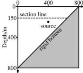
[image:3.595.223.362.244.365.2]The geometry of the boundaries and the definite conditions are needed for solving the wave equation. We test our implementations on an ideal wedge problem in this paper. In this problem, a pressure-release sea surface and a rigid or pressure-release bottom constitute the main boundaries of the 2D wedge. Both the surface and the bottom are perfectly reflecting boundaries and in the opposite the left boundary has to be set to a non-reflecting (absorbing) boundary. Although, in the real ocean environment, the wedge angle is very small, in this paper, we set it to 45° for simplicity. As shown in Figure 1, there is a line source situated in the wedge.[7]
Figure 1. The sketch of the ideal wedge environment. The dashed line indicates the sampling area.
The definite conditions include the boundary condition and the initial condition. The boundary conditions describing the sea surface, bottom and the left vertical boundary are listed as follows:
·The rigid boundary: n
0
p
·The pressure-release boundary: p0
·The non-reflecting boundary: pt
(
p
)
0
[image:3.595.178.419.542.678.2]The numerical schemes and the solver and preconditioner in OpenFOAM used in describing and solving the wave equation from the boundary and initial conditions are listed in Table 1 and Table 2.
Table 1. Numerical schemes and boundary conditions.
In order to get the frequency domain results, the post-processing frequency analysis method should follow the steps listed in Figure 2.
Figure 2. Post-processing frequency analysis method.
·Solving and sampling. The time domain results of the wave equation are the $p$ values on each mesh point at each time step. It does not give an explicit description to the frequency distribution of the solution. Along the dashed line in depth of 150m shown in Figure 1, the frequency analysis method samples the p value in every time step and output them to a text file.
·Output. It collects the full time domain simulation results of specified mesh points at all time steps. The output process gives time series of s value on each specified mesh point.
·Serial transformation. We plot the results outputted from the sampling step, and manually mark the moment at which the sound field reaches its periodic status. Then cut the time series for temporal -frequential transformation. The transformation step calculates the distribution on finite frequency points from the time series on the mesh points, and output the maximum of the distribution as the transmission loss. This step is implemented in a third-party software, and its execution is serial.
The post-processing frequency analysis method mentioned above has three main disadvantages:
·The non-restricted sampling step results in the booming of the I/O data scale. According to the statistics included in Section 4, writing data of 820 cells from 40,000 time steps to the file will bring the simulation an execution time increase by 3% to 8%.
·The calculations of the Fourier transform on multiple spatial points are independent of each other. These calculations are naturally suitable for task level parallelism. However the transformation is restricted to serial by the third-party platform on which it is based. Some experiments show that the transformation of the data from 820 cells and 40,000 steps costs over 60 seconds.
·From the graphic results of the time domain simulation we can see that it takes some time for the sound wave from a point source to spread out the entire field. In the experiments in this paper, this time period lasts about 10,000 time steps. The results before the sound field reaching stability are not only no use but also harmful for possibly bring extra errors to the transformation[10].
The Basis of the Embedded Frequency Analysis
On top of the discussions in Section 2.2, we present the following modifications of the post-processing frequency analysis method.
We add a cache mechanism to the sound propagation solver in OpenFOAM for recording p value on specified cells. We implement a fast Fourier transform function in OpenFOAM, to calculate the frequency distribution from the time series kept in the cache after all time steps finished. This calculation is paralleled under the instruction of /system/decomposePar.
In the sampling step we add restrictions. They keep the sampling operation in the specified time period after the non-stable stage of the propagation of the sound wave and they remove the repeating periods of the stable status.
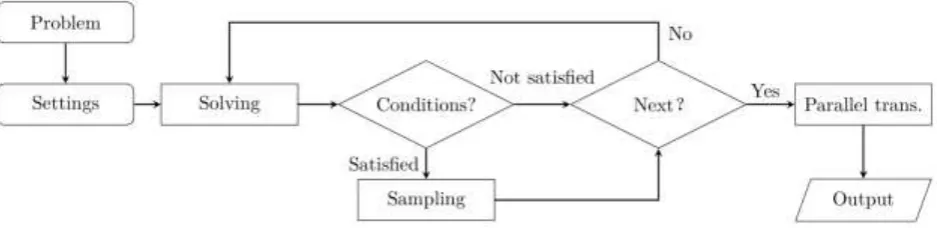
Figure 3. The embedded frequency analysis method.
·Settings. Set the restrictions to the sampling step. They indicate in which cells and time steps are we interested.
·Next. This decision module starts the next step of the loop which solves the wave equation. The sampling step locates in that loop.
·Conditions and Sampling. The condition is set in the Settings step. If the number of current time step satisfies the condition, then the main function invokes the sampling function to record $p$ data.
·Parallel transformation. After finished the time domain simulation, the program invokes the transformation function on each parallel threads.
·Output. Write the frequency domain results to a file.
The Implementation of the Embedded Frequency Analysis
In this section we implement the embedded frequency analysis tool and modify the direct simulation platform. The main work includes fast Fourier transform (FFT) based on OpenFOAM, the cache mechanism for recording the time domain data and the restrictions to sampling.
An O(N log2 N) complexity FFT algorithm includes two operations. One is called the bit-reverse
If the length of the input of Algorithm 2 does not a power of two, we should add zeroes to the tail of the sequence to extend it. In the step of finding the maximum norm of the output of function void FFT (float xReal[], float xImag[], int n), we employ the fast inverse square root algorithm from Lomont[12].
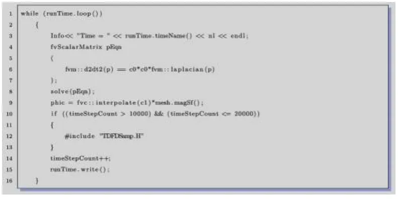
In this code segment, the integer variable timeStepCount is used as the counter of time steps.
Results
The Platform and the Parameters
The Platform: In the experiments we use an HPC cluster situated in the State Key Laboratory of High Performance Computing. This computing platform consists of hundreds of computing nodes and each node contains 12 Intel Xeon 2.1 GHz E5-2620 CPU cores and a total memory of 16 GB.
The Ideal Wedge Problem: The ASA ideal wedge wave guide sound propagation problem shown in Section 2.
The Parameters: The parameters include the sound speed in the wave guide c = 1500 m/s, the density of the media = 1.0 g/m3, the wedge angle of 45°, the source location of 400 m in range and 200 m in depth. The periodic source problem uses a source with 25-Hz frequency.
Verification and Validation
In this experiment we compare the results of the embedded frequency analysis with the calculation based on the third-party software[13]. The comparison indicates that the results of the function void FFT (float xReal[], float xImag[], int n) match well with those given by Mathematica. The embedded tool is accurate enough to replace those third-party tools in the frequency analysis.
Efficiency Statistics
In this section we present the experiments on the studies of executing efficiency of the embedded frequency analysis. We time 6 executions including the direct time domain simulation (Tsolve), the file
writing sampling (TsampW rt ), the non-writing sampling ( noW rt samp
T ), the post-processing transformation (Ttranspost), the embedded transformation (
emb trans
T ) and the sampling and transformation with restrictions (Tsres&t). We time these operations under serial and 4 degrees of parallelism on a 508,800 cells mesh for 40,000 time steps.
Figure 4 illustrates the time cost Tsolve of solving the ASA problem in OpenFOAM without
[image:7.595.100.496.69.267.2]Figure 4. The execution time of solving the wave equation in time domain.
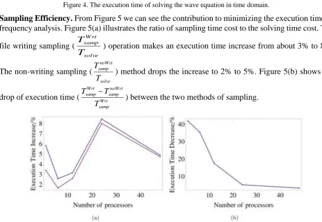
Sampling Efficiency. From Figure 5 we can see the contribution to minimizing the execution time of frequency analysis. Figure 5(a) illustrates the ratio of sampling time cost to the solving time cost. The
file writing sampling (
solve W rt samp
T T
) operation makes an execution time increase from about 3% to 8%.
The non-writing sampling (
solve noWrt samp
T T
) method drops the increase to 2% to 5%. Figure 5(b) shows the
drop of execution time ( Wrt
samp noWrt samp Wrt
samp T
T
T
) between the two methods of sampling.
Figure 5. The effect on time overhead of sampling: (a) The increase of execution time using file writing and non-writing sampling tools. The blue line indicates the file writing method, the red line indicates the non-writing one. (b) The decrease
of time overhead using non-writing sampling method comparing with the file writing one. (
Wrt samp noWrt samp
T T
)
[image:8.595.58.522.225.545.2]Figure 6. The effect on decreasing time overhead by embedding the transformation tool into OpenFOAM. ( post trans emb trans T T
)
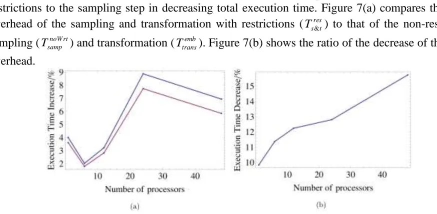
The Effect of the Restrictions to Sampling. Figure 7 mainly present the contribution of the restrictions to the sampling step in decreasing total execution time. Figure 7(a) compares the time overhead of the sampling and transformation with restrictions (Tsres&t) to that of the non-restricted sampling (TsampnoW rt) and transformation (Ttransemb). Figure 7(b) shows the ratio of the decrease of the time overhead.
Figure 7. The effect of restrictions to sampling: (a) The comparison between restricted frequency analysis and the non-restricted one. The blue line indicates the non-restricted situation, the red line indicates the restricted situation. (b) The
decrease of time overhead on sampling and transformation after set restrictions to the sampling step.
Conclusion
In this paper we analyze a underwater sound propagation direct simulation and frequency analysis technique based on OpenFOAM and its post-processing tools. We present improvements to the technique and compare the modified technique with the original one on accuracy and efficiency. The discussions and experiments are based on the ideal wedge wave guide sound propagation problem introduced by Acoustic Society of America.
[image:9.595.68.506.260.474.2]In conclusion, the analysis on the underwater sound propagation direct simulation and frequency analysis technique based on OpenFOAM is correct, and the improvements and there implementations are effective.
Acknowledgements
This project is supported by National Natural Science Foundation of China (Grant No. 61303071) and the open fund from the State Key Laboratory of High Performance Computing (Nos. 201503-01 and 201503-02).
References
[1] R.H. Zhang, Progress in research of ocean acoustics in China, Physics, 23.9 (1994) 513-518. [2] X.L. Jin, The development of research in marine geophysics and acoustic technology for submarine exploration. Progress in Geophysics, 22.4 (2007) 1243-1249.
[3] W.Y. Luo, C.M. Yang, J.X. Qin, R.H. Zhang, Benchmark solutions for sound propagation in an ideal wedge, Chin. Phys. B, 22.5 (2013) 054301.
[4] A. Tolstoy, 3-D propagation issues and models, J. Computational Acoustics, 4.3 (1996) 243-271. [5] R.A. Stephen, Solutions to range-dependent benchmark problems by the finite-difference method, J. Acoust. Soc. Am. 87.4 (1990) 1527-1534. J. Sound and Vibration, 45.4 (1976) 495-502.
[6] M. Petyt, J. Lea, G.H. Koopmann, A finite element method for determining the acoustic modes of irregular shaped cavities.
[7] L.B. Felsen, Quality assessment of numerical codes, part 2: benchmarks, J. Acoust. Soc. Am. 80 suppl. 1 (1986) S36-S37.
[8] M.J. Lighthill, On Sound Generated Aerodynamically. I. General theory, Proceedings of the Royal Society of London A: Mathematical, Physical and Engineering Sciences. 211.1107 (1952) 564-587. [9] F.B. Jensen, W.A. Kuperman, M.B. Porter, H. Schmidt, Computational Ocean Acoustics, Springer Science & Business Media, 2000.
[10] W.H. Press, Numerical Recipes 3rd Edition: The art of scientific computing, Cambridge University Press, 2007.
[11] T.H. Cormen, C.E. Leiserson, R.L. Rivest, Introduction to Algorithms, MIT Press, 2007. [12] C.Lomont, Fast inverse square root, Technical Report-315, (2003) 32.