Symptom Proximity in Diagnostic Problem

(1)

Symptom Proximity in Diagnostic Problem

Otakar Kˇr´ıˇz

Prague, Czech Republic

Abstract

An algorithm SP (= Symptom Proximity) is suggested for solving discrete diagnostic problem. It is based on probabilistic approach to decision-making under uncertainty, however, it does not use knowledge integration from marginal distributions.

Keywords

Probabilistic Decision Making, Diagnostic Problem

1 Informal analysis

The ability of decision-making belongs to the most im-portant mechanismus build in complex organisms. Optimal strategies for decision-making determine the success or even survival of different animal species (Darwin theory), trading companies or individual patients.

As mentioned e.g. in [5], decision-making can take place on a purely intuitive basis (i.e. an individual decision is pro-vided by a genetically inborn mechanism or it can be given by experience acquired during the life span of a decision-maker and stored in neural structures of his brain ). Or, decision-making can take place on the basis of a more considered strat-egy and in the framework of a formalized theory.

When collecting a large number of facts relating to a situ-ation, there appears a point, in certain phase, where facts are ”abstracted” to a piece of knowledge. (The process is refered to as hegelian dialectic concept of ”quantitative change leads to qualitative change”.) Knowledge is usually expressed in form of sets of implications. Then, in the context of decision-making, observed facts (calledevidences) on an individual object are used as antecedents and the required decision is, hopefully, provided via laws of logics from the succedents (of the implications). However, even this approach involves implicitely certain degree of uncertainty (e.g. when to switch from facts to a law/knowledge).

The tolerable precision is domain dependent. In physics, a theory must explain data with precision to six decimal posi-tions. In soft sciences, models are less demanding.

Therefore, one can generalize that decision-making cannot be separated from uncertainty. Partially, it is due to the

men-tioned ”ever present lack of data” and partially, there exists an ”uncertainty” which of formal theories of uncertainty to use as a model. Even in probability, taken usually as a nor-mative theory (for uncertainty), there exist alternatives (see e.g.[4]).

One of the most fruitful lines in probabilistic decision-making (see subsection 2.1) can be divided into four phases: First, select less-dimensional distributions, considered as marginalsof atheoretical joint distribution, as input knowl-edge.

Second, one can construct (integrate) an explicit formula for thejoint distribution. It can be done via strong assump-tions like conditional independence between marginals ex-pressed asgraph models.

Third, given anevidenceabout an object (i.e. measured on the object), the formula is reduced (marginalized) to a sim-pler form where theevidencecan be directly applied.

Fourth, the ”best” decision is the one that yields largest conditional probabilityondiagnosis variable(i.e. containing decisions) given the observedevidence.

The topic of this paper is a method/algorithm SP that does not use the marginals (and assumptions about their con-ditional independence) and finds an approximation of the largest conditional probability directly from the data (called statistical file in the sequel and defined in subsection 2.3).

Let us suppose that both models (i.e. ”marginal ”one and SP) are finite and discrete.

( Explicitly, we do not consider e.g. family of log-linear dis-tributionsand noestimationof theirparametersfrom the sta-tistical file takes place as is usual instandard statistics).

There is a discrete number ofsymptom variables, discrete number ofsymptoms in range of eachsymptom variable, dis-crete number of diagnoses/decisions and finite number of ob-jects in thestatistical file (representing knowledge).

It should be stressed that if one uses the term ”measured” it should be interpreted as ”measured and discretized”. E.g. biochemical values, though continuous, are reduced to di-chotomies (greater or less than a threshold) or tridi-chotomies (”standard values”, ”too low”,”too high”).

(2)

symptom variables.

In ”marginal approach”, thejoint probabilityformula is in-tegrated once forever frommarginals(elicited, in their turn, from a ”learning”statistical file).

Then, thisuniqueformula is used for eachevidence avail-able for the object/patient/case.

Whereas, ”marginal models” construct anunique approx-imative distributionof anuniquetheoretical joint distribu-tion, the SP-model uses for decision-making anadhoc ap-proximation of conditional probability ( derived from the unique theoretical joint distribution). (This link is estab-lished by the supposition that thestatistical filewas generated (by nature?) according to a theoretical joint distribution.) Thisadhocapproximation of conditional probabilityis gen-erated freshly from scratch for each set ofsymptom variables (carryingevidencemeasured on the object/patient). (In other words, the termadhocrelates to a disclosed set ofsymptom variables.)

The aim of SP is not to ”predict” the shape of aposteri-ori probabilitiesof all considered diagnoses, but only to find the most probable diagnosis/decision and even the numerical value of itsaposteriori probabilityis not important. In other words, what matters is just the first place in this ranking.

What is new ?

In eighties, it was believed that whereas the data (i.e. sta-tistical file) is not sufficient for estimating thejoint distribu-tion, it should do for less-dimensional tables (i.e. supposed marginals). Moreover, these marginals were considered as given externally and reliable as ”incorporated truth”. Beside being given from outside, themarginalswere just few. One might use amarginalfor integration or leave it out. Not ask for new ones! The argument that marginalscannot be ob-tained otherwise than from the data was not paid sufficient attention to. If it would have been taken into consideration, one could ask for moremarginals, but, at the same time, it would raise questions like ”How manymarginalsshould we ask for?” and ”What would be the best composition of those marginals?”.

The central notion was theapproximationof thejoint dis-tributionwhereas it is theapproximation of conditional prob-ability that SP takes as its ”flag ship”. At the same time, the role of disclosedsymptom variablescarryingevidenceis stressed for SP, as well. Then, the detour ”integration to joint distribution” and subsequent marginalization is not needed any more.

A specific methodology based on proximity (of vector of evidences and respective vectors constructed from cases in thestatistical file) in space ofsymptom variablesis used in SP algorithm.

To explain the theory of the SP algorithm, simplemetrics is introduced in section 3.

As details matter and redundancy is preferable to ambi-guity, the essence of the algorithm SP is described twice in section 4.2. Namely, via a flowchart (see Figure 1.) and via a code written in a symbolic language. The latter description makes possible to derive computational complexity for SP in section 5.

However, the real strength of SP lies in the fact that this

approach is fast enough to operate on large statistical files with large number ofsymptom variables.

As far as decision quality is concerned, the situation is not so transparent. On one hand side, it is possible to construct examples where SP dominates the ”marginal approach”. It may happen when inputmarginalsare ”at wrong position” to the disclosed symptom variablescarryingevidences. How-ever, in general, the dominance of SP cannot be directly proved and one can only compare SP and one of many pos-sible ”marginal” algorithms, with different sets ofmarginals and for differentevidence-carryingsymptom variables. And it has to be done in many combinations. This ”branching ex-pansion” is multiplied by two when we consider two testing techniques. First, ”testing” and ”learning”statistical filesare identical. Second, the ”leave one out” technique, described in section 6, is used.

The final impression (from this multicriterial decision-making) is that SP does very well. It is based on experience from many comparative runs. If it is not dominant, SP be-longs to Pareto optimum, at least.

It should be noted that SP does not use theempirical distri-butionderivable from thestatistical file. (The ”mass” of the empirical distributionis concentrated only in theatomsof the definingset algebrathat appears in cases from thestatistical fileand it is zero anywhere else).

One may ask why this line of research (i.e. ”without marginals”) was not followed as a main stream before?

In my opinion, during the last decades, external material conditions (computerization and existence of large databases) changed a lot. In the meantime, the original paradigm was re-fined and improved by many researchers. The model became so rich, successful and invested in that the inertia prevented an investigation if basic suppositions cannot be weakened.

2 Specific statement of the problem

2.1 Historical background

(3)

specific solution was suggested even before in [2]. Different models, connected with names like Lauritzen, Spiegelhalter, Dempster, Shafer, Pearl, Dawid, were studied with assump-tions about conditional independence of variables appearing inP that helped to integrate the marginals. At present, there exist professional software packages (e.g. Hugin) supporting the decision-making on commercial basis. As, beside differ-ent algorithms, even the selection of proper marginals may be a problem of its own (see e.g. [9] and [10]), this paper tries to study an alternative to the marginal approach.

2.2 The layout of the paper

1. Informal (i.e. without notation) analysis of the diagnos-tic problem in probabilisdiagnos-tic setting is given in section 1. 2. There are historical reminiscences explaining the posi-tion of the suggested method in a broader context in sub-section 2.1.

3. Basic notions are defined including the formulation of the diagnostic problemand describing the role of the statistical fileFin subsection 2.3.

4. The essential features of the algorithmSPare laid down in section 3.

5. Realisation of SP is described in section 4 via a flowchart (in subsection 4.1) and via symbolic program-ming language (in subsection 4.2).

6. On the basis of the latter description, computational complexityCSP of SP in terms of ”length” l = |F |

of the fileFand of its ”width”n=| {ξ1, ξ2,· · ·ξn} |is

estimated and verified experimentally for different val-ues oflandwin section 5.

7. ”Discernment power” ofSP(i.e. absolute values or per-centage of wrong classifications ) is tested for different ”apertures” ( sets of symptom variables whose values are disclosed toSP as evidence). Testing is performed both via method ”leave one out” as well as on all data in simulation runs. The results are compared with a simple marginal-based algorithm under the same testing condi-tions in section 6.

8. In section 7, there are features ofSP sorted as ”pros” and ”cons”. Then, there are two open questions sug-gested for further investigation and finally, there is a summarizing conclusion.

2.3 Basic notions and notations

Let(Ω,X, P)be a probabilistic space,η=ξ0,ξ1,ξ2, . . .ξn

be finite sets and ξr : (Ω,X, P) −→ (ξr,2ξr)forr =

0,1,2,· · ·nbe measurable functions.

Though the topic is defined in a formal way, the names of objects in the universe of discussion (e.g. diagnosis, symptoms etc.) are taken from the field of medicine to give

them a semantical interpretation and ease up understanding of basic notions and character of their interaction.

The mutual behaviour of all random variables

η, ξ1, ξ2· · ·ξn is described by a theoretical joint

proba-bility distributionPη ξ1ξ2···ξn.

Decision making under uncertainty with probabilistic back-ground can be interpreted as the diagnostic problem with the following formulation:

Diagnostic problem:Find the diagnosisd(s1, s2· · ·sn)∈η

that is the most probable (according to thePηξ1,ξ2···ξn) on the

set{ω ∈Ω|ξ1(ω) =s1 &ξ2(ω) =s2& · · ·ξn(ω) =sn}

for a given (i.e. observed) arbitrary combination

(s1, s2· · ·sn) of values of symptom variables from the

cartesian product Ξ = ξ1×ξ2×. . .ξn. If we wish to

predict the values of diagnostic variable η, the conditional probability Pη|ξ1ξ2...ξn (derivable from Pη ξ1ξ2...ξn) should

be used instead ofPη ξ1ξ2...ξn.

Optimal decision: The value of diagnosis d from η that should be selected if the values of symptom variables are (s1, s2· · ·sn) to keep the wrong classifications of d

as low as possible), called Bayes solution, is for each

(s1, s2· · ·sn) ∈ ξ1×ξ2×. . .ξn

given by the formula

dopt(s1, s2· · ·sn) = argmax d∈η

Pη|ξ1ξ2...ξn(d|s1, s2· · ·sn)

(1) So far the theory. Unfortunately, in the ”real world”, we are never given the theoretical distributionPηξ1ξ2···ξnin full and

directly. To compensate for this, we expect to have some in-direct information aboutPηξ1ξ2···ξnthat will be called

knowl-edge baseand denoted byK. It is done by postulating a set of conditions that we believe the theoreticalPηξ1ξ2···ξnfulfills.

Marginal problem: Using the concept of marginal prob-lem, see [6], knowledge base K is given as a set of ”low-dimensional” distributions (i.e. number of variables in the distribution does not exceed e.g. 10. ), postulated as theo-reticalmarginal distributionsof thePηξ1,ξ2...ξn. Beside the

marginals, there are usually made assumptions about condi-tional independence holding between groups of random vari-ables. It is interesting that the topic was so attractive that it was addressed in several waves, usually after 20 years. Orig-inal and interesting ideas were not just the product of the last two decades but go back much deeper. See e.g. [2], [6],[3], [1]. Instead of the unknownPηξ1ξ2···ξn, we try to construct

(from the marginals) its suitable approximation Pˆηξ1ξ2···ξn

that could play its role in the formula (1).

If existence of marginals is postulated, it is natural to ask where do they come from. Therefore, another notion should be specified.

Statistical fileF: Let(ω1, ω2,· · ·ωs)be a sequence, where

(4)

fromΩ,

then the sequence (η(ωl), ξ1(ωl), ξ2(ωl)· · ·ξn(ωl))sl=1

of points in cartesian product η ×ξ1 ×ξ2 ×. . .ξn is a

statistical fileF of sizes(i.e. s=|F |) and(F)ris ther-th

member of the sequenceF.

There exists a taciturn assumption that decision making about a concrete case (patient) should be very fast (about 1 sec/pers.). On the other hand, longer time (e.g. hours of CPU time) devoted to selecting and populating the marginals (in the learning phase) is tolerable. This may be one of the reasons why the ”marginal approach” is the standard way. However, using marginals for ”integrating”Pˆηξ1ξ2···ξnand

its subsequent conditioning need not be mandatory for solv-ing the diagnostic problem.

3 Basic idea of SP algorithm

An algorithm, called SP ( = Symptom Proximity), tries to construct necessary conditional probabilities directly from available statistical data file F. Basic idea of SP can be explained by the assumption ”Patients with similar symptoms should have a similar diagnosis”. Hence, the name of the algorithms SP interpretes the similarity as a proximity in the sense of a very natural metrics.

Proximity metricsρ:

ρ: Ξ×Ξ−→R (u,v)7−→n−

n

X

i=1

δ( (u)i,(v)i)

whereδ(·,·)is the Kronecker function and (u)i is the i-th

component of the sequence uThe mapping ρ is a metrics (i.e. reflexivity, symmetry, triangular inequality) on Ξthat can be used for defining equivalence classes onΞ. For each fixedv∈Ξ, there existn+ 1setsC0(v), C1(v),· · ·Cn(v),

whereCk(v) ={u∈Ξ |ρ(u,v) =k}.

The next step is to estimateP(Ck(v)). It can be done, in a

natural way, using available data ( i.e. the statistical fileF).

P(Ck(v)) =

|F |

X

j=1

δ(ρ(((F)j)Ξ,v), k)/|F |

where(F)jis the j-th vector from fileFi.e.(F)j ∈η×Ξ.

Similarly, ((F)j)Ξ is that part of the j-th vector(F)j that

corresponds to symptom variables i.e.((F)j)Ξ∈Ξ. We are

interested in the setCk(v)with smallestk but at the same

time such thatP(Ck(v))>0. Let us denote this optimalk

ask0

Finally, the conditional probabilityP η|Ck0(v)(d|v)ofηon Ck0(v)can be defined.

To shorten the shape of the final expression for the

P η|Ck0(v)(d|v), an auxillary variable D(F,v, k0, d)will

be introduced. It denotes the number of cases (patients) from the statistical file F that ”belong” to the equivalence class

Ck0(v)and at the same time they have the diagnosisd

D(F,v, k0, d) =

|F |

X

j=1

δ(ρ(((F)j)Ξ,v), k0)δ(((F)j)η, d)

(Similarly according to the above used notation, ((F)j)η

stands for the value of the diagnosis that is in the j-th vec-tor of the statistical fileFi.e.((F)j)η∈η. )

Then,P η|Ck0(v)(d|v)is defined by

P η|Ck0(v)(d|v) = D(F,v, k0, d)/(|F | ·P(Ck0(v)))

If v = (s1, s2,· · ·sn) ∈ Ξ, we may approximate

the conditional probability Pη|ξ1ξ2...ξn(d|s1, s2· · ·sn)

(1) can be applied as the decision rule in the SP algorithm. The algorithm SP is presented in a symbolic programming language in section 4.2. The complexity of the algorithm SP will be defined, in section 5, as a function of size|F |of the data fileF and as a function of numbernof symptom vari-ables. The complexity is verified on real data by measuring time required for making decision for one person.

The decision quality (or discernment power) is dealt with in section 6. In principle, it is the number of wrong classifica-tions what is measured. However, it may be defined more formally:

LetL ⊂ F,v ∈ Ξ. Further, let SP(L,v)∈ ηdenote deci-sion of SP when evidence (about a patient) isvand algorithm SP has the ”learning” fileLat his disposal. Then, ”discern-ment power” of SP can be measured by percentage of wrong classifications either as

100



1−1/|F |

|F |

X

j=1

δ(SP(F,((F)j)Ξ),((F)j)η)

 

or with the formula

100



1−1/|F |

|F |

X

j=1

δ(SP(F \(F)j,((F)j)Ξ),((F)j)η)

 

.

This second approach is referred to as ”Leave one out” technique. (There are more details on the technique in section 6.)

The results will be compared with one simple algorithm using the ”marginal approach” in section 6.

4 Detailed description of SP

(5)

As mentioned above in section 2, SP algorithm is described twice. Namely, via a flowchart (see Figure 1.) and via a code written in a symbolic language.

Strictly speaking, realization of an algorithm is an exe-cutable file (i.e with extension.exe) that is ”understood” e.g. by any PC.

Less strictly, realization of an algorithm is syntactically and semantically correct text file ”written” by a man-programmer in a general purpose programming language (like Fortran, C ,C++, Visual Basic) that is ”understood” by a compiler of the respective language. (This text file has extensions like.for, .c, .vbs.)

Next level is symbolic language. It is an abstraction of general purpose languages. It is ”written” by man and it can be ”understood” by another man to the extent that he/she can rewrite it to correct text in general purpose language.

The last common representation of an algorithm is its flowchart. It is a ”text” written by man-programmer in graph-ical language form. It has to be ”understood” by another man. It has conventional structures like action blocks (rectangles), decision blocks (rhombus or trapezoid) and lines where ar-rows determine the ”flow” of the program. Some symbols are overloaded. E.g. symbol ”=” is interpreted as an assign-ment in action blocks whereas it is a relational operator in decision blocks.

To summarize, there is always potential place left for ambi-guity and misunderstanding. Therefore, both descriptions of the realization are used in parallel and they are supplemented by informal comments that explain semantics of used struc-tures (in context of theoretical foundations of the algorithm). There is a slight functional difference between the flowchart and the symbolic language descriptions of the SP algorithm.

The flowchart describes entering one statistical file L

(from the problem area) and entering asequence of sev-eral newevidencesv for which their optimal diagnoses are calculated.

In the symbolic language, there is a body of afunctionSP where onlyone givenstatistical fileLand onlyone evidence vare entered asparameters.

Then, the corresponding diagnosis dopt(v) is calculated

and returned when thefunctionSP ends. The difference is only a formal one and the essence of SP algorithm is the same.

4.1 Flowchart of SP

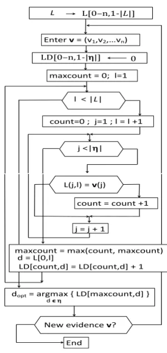
It represents the activity of the algorithm in a simplified form. It is a link between the theory and the realization. Therefore, the symbols from both ”worlds” are used. E.g. the first action block describes the filling of the array L with values from the statistical file denoted as L to stress it is for ”learning”. Names of the symptoms, usually in form of text strings, are densely coded into integers. Denotation L[0−n,1− |L|]says that two-dimensional array L hasn+ 1

positions in the first dimension. (Position ”0” is used for stor-ing diagnoses, positions ”1” to ”n” are for storstor-ing values of symptom variables). The second dimension is for indexing

individual records fromL. Variablemaxcountcorresponds to

k0via definitionk0=n−maxcount. There are three loops

in flowchart which are realized asfor-cycles in the symbolic language. Filling the two-dimensional array LD with zeroes takes place anytime newevidencev is entered. In the end, after running through the whole L matrix, the array element LD(i,j) contains the numberD(L,v, n−i, dj). It is easy to

see that elements of the matrix LD are integers and their sum is|L|.

L L[0–n,1-|L|] |||

0

[image:5.595.332.496.223.568.2]

maxcount = 0; l=1

l < |L|

count=0 ; j=1 ; l = l +1

j <|η|

0

|||

LD[0–n,1-|η|]

|||

Enter v = (v1,v2,…vn)

L(j,l) = v(j)

count = count +1

j = j + 1

maxcount = max(count, maxcount) )

LD[count,d] = LD[count,d] + 1 d = L[0,l]

dopt = argmax { LD[maxcount,d] } d 𝞊 η

New evidence v?

End

Figure 1.Flowchart of SP.

It would be possible to calculate the approximation of con-ditional probability P η|Ck0(v)(d|v) of η on Ck0(v). (It

can be done by normalization of the row LD(maxcount,*) of the array LD. i.e. by dividing elements in the row LD(maxcount,*) by their sum.) However, as we are inter-ested only in the ranking, this normalization is not necessary and we look for dopt by looking for maximal value in the

row LD(maxcount,*) of matrix LD, only. That way, we save computational time by skipping unnecessary actions.

(6)

4.2 Description of SP in a symbolic language

SP algorithm can be used in different roles. It may be a simple ”one-shot” making, repeated decision-making for different apertures (sets of symptom variables whose values are disclosed to SP as evidence), using SP

in a general testing scheme or it may be adapted to specific testing via ”Leave one out” technique.

Instead of using one highly parametrized form ofSP al-gorithm, it seems better, for didactical reasons, to use several stand-alone modifications. However, only the most simple version, under the namefunction SP, will be presented in this paper. Specific modifications built on its basis ( and en-titled SPL and SPA) will be mentioned in other sections. The following symbolic description is kept as simple as possible. First, though the variables have their specific denotation reflecting their semantics, they are coded as integers or arrays of integers to makeSP faster.

Second, tests and resulting exceptions in inconsistent situ-ations such as|L|= 0or|η|= 0are omitted !

Third, this version of SP algorithm is defined for all n

available symptom variables. However, it can be easily mod-ified if not values of all symptom variables are known, but if only some of them are provided as evidences (i.e. in case of smaller aperture).

Function SPreturns the valuedopt(v)for each given v =

(v1, v2· · ·vn) ∈ ξ1×ξ2×. . .ξn

1 functionSP(v)

2 readL −→ L(0−n,1− |L|) 3 forj= 1,|η|

4 fori= 0, n

5 LD(i, j) = 0

6 nexti

7 nextj

8 maxcount= 0

9 forl= 1,|L|

10 count= 0

11 forj= 1, n

12 ifL(j, l) =v(j)then

13 count=count+ 1

14 endif

15 nextj

16 ifmaxcount < countthen

17 maxcount=count

18 endif

19 d=L(0, l)

20 LD(count, d) =LD(count, d) + 1

21 nextl

22 max= 0;dopt= 0

23 forj= 1,|η|

24 val=LD(maxcount, j)

25 ifmax < valthen

26 max=val

27 dopt=j

28 endif

29 nextj

30 SP =dopt

31 end

Comments to the code ofSP:

l.1expresses thatSP is a functionSP : Ξ −→ η i.e. ac-cepts as argument the vectorvand returns the optimal diag-nosisdopt(v).

l.2 learning fileLis stored in an array L. The value ”0” in first dimension is for values ofη.

l.3 - l.7sets zero values to the array LD (level distance) where metrics will be stored in the sequel.

l.9 - l.21 For each l ∈ L, number of symptom variables with coinciding values (symptoms) is calculated in the vari-able count. Increasing LD(count, η(l)) by one increases chances of diagnosisη(l) to become optimaldoptif the

de-cision should take place at the levelcount.

l.16 - l.18stores inmaxcountthe up-to-now achieved max-imal number of coincidences.

l.23 - l.30 finds in LD(maxcount,j) such diagnosis dj that

would, on the levelmaxcount, define the winning dignosis

dopt. Naturally, if the number of cases fromLis small (and

that would result in objections from statistical point of view), it is possible to perform search for optimal diagnosis on a level countsmaller than maxcount that would have more objects than levelmaxcount. Or even, it is possible to sum

LD(ct, j)forct=counttomaxcountin an array D(1-|η|) and search fordoptin this array. (However, this modification

ofSPis not available in the presented version.)

The link of the code with previous formal description may be made more clear if we realize that the variablemaxcount

is related tok0. However, their roles are reversed in the sense

thatmaxcountis the number of coincidences (of symptoms from u and v) and should be as close to n as possible, whereask0 is proximity (in the sense of the metricsρ) and

should tend to zero. Further,v(j)is(v)jand the value in the

arrayLD(maxcount, j)stores theD(L,v, k0, dj).

5 Computational complexity

It should be mentioned that experimenting with algo-rithms was performed on a statistical fileF, from the field of rheumatology with 1089 patients. Diagnosis variable η

contained 4 diagnosis and there were 34 symptom variables whose ranges had cardinalities from 2 to 9. That way, no generation of artificial examples was necessary. Neverthe-less, this choice has no influence on the substance ofSP. Complexity CSP of SP algorithm can be mesured with

respect to the number of symptom variables n, number

|L|of objects in the learning fileL and with respect to the number |η| of diagnoses i.e.CSP = C(n,|L|,|η|). Due

to the simple structure ofSP,CSP can be estimated directly:

l.2 c1∗n∗ |L|

l.3 - l.7 c2∗n∗ |η|

l.9 - l.15 ˙ c3∗ |L| ∗(n+c4)

l.23 - l.29 c5∗ |η|

—————————————————————

(7)

[image:7.595.68.258.105.234.2]

Table 1.Computational time dependence on lengthm=|F |of fileF

m Tread Ttotal Tdecision

1000 31 msec 1 sec 10 msec

2000 60 msec 2 sec 20 msec

5000 156 msec 25 sec 50 msec

10000 343 msec 100 sec 100 msec

20000 687 msec 400 sec 200 msec

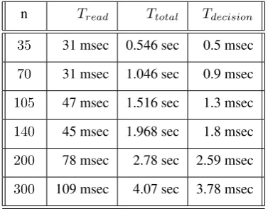
Table 2.Computational time dependence on widthnof fileF

n Tread Ttotal Tdecision

35 31 msec 0.546 sec 0.5 msec

70 31 msec 1.046 sec 0.9 msec

105 47 msec 1.516 sec 1.3 msec

140 45 msec 1.968 sec 1.8 msec

200 78 msec 2.78 sec 2.59 msec

300 109 msec 4.07 sec 3.78 msec

The assumption of linearity (c1, c2· · ·) is a bit simplifiction

and valid only for small ranges ofn,|L|,|η|. If the ranges are greater, then effects like ”paging” of memory, the way files are stored in a concrete file system (e.g. FAT 32 or NTFS) and variables used for storing the ”coding” numbers may come in play. E.g. values ofηare stored in variables of typeinteger*1and therefore should not exceed 256. Therefore, instead of looking for explicit values forc1,· · ·c5,

direct measurements are documented in Table 1 where length

|L|of L varies from 1000 to 20000 and in Table 2 where width n of L varies from 35 to 300. Corresponding files

L(e.g. L(70,1089)or L(35,20000)) were generated from originalL (i.e. L(35,1089)) by repeating respective rows and columns. In the Tables 1 and 2, column Tread

con-tains time necessary to readL. ColumnTtotalincreases with

square power of|L|as it is the time necessary for|L| deci-sions. WhenTtotalis divided by|L|, then the times in column

Tdecisionare always below 1 sec and therefore completely

acceptable. Based both on analysis and direct measurements, complexity ofSP is not a problem. Therefore, the limiting factor for better discernment power ofSP is an externality i.e. experts should provide bigger data in form of a fileF(or

L).

6 Simulation results

This section should reflect the decision-making quality of SP via simulation results. Simulation is performed on the data mentioned in the beginning of section 5. Though the fol-lowing example is very simple, it may reveal interesting facts when comparingSPand the decision-making algorithmA4

(from [7] and mentioned in [8]) that can serve as a simple representative of marginal-based algorithms. Let knowledge baseKBconsist of 3 marginals i.e.KB={m1, m2, m3}.

The marginals can be defined by their ”generating” symp-tom variables (besides implicitely supposed diagnosis vari-able η). Underscoring of symbol for a marginal denotes the set of ”generating” symptom variables. E.g., if m1 =

{ξ25, ξ33}, thenm1=Pηξ25ξ33.

Then,KBused for testing was defined via

m1={ξ25, ξ33}, m2={ξ26, ξ32}, m3={ξ27, ξ33}

.

The ”testing environment” provides an easy way to manipu-late with ”inputs” to the decision-making algorithm.

First, it makes possible to remove marginals from KB and second, not all symptom variables, from n possible ones, need to be revealed as ”evidences” to decision making-algorithmSP orA4. We testedSP orA4 alongside for 8 different situations s1, s2,· · ·s8 described in Table 3. E.g.,

the expression{m1, m3} ∩ {ξ1−ξ33}(in column ”marginals

∩ variables” of Table 3) stands for situations2 whereKB

consists only of marginals {m1, m3} and values of all 33

symptom variables{ξ1−ξ33}are submitted as ”evidences”

to the SP andA4. (Naturally, {m1, m3} has impact only

on A4, whereas {ξ1 −ξ33} influences both SP and A4

). Column ”active variables” in Table 3 contains symptom variables whose values have influence on A4 as result of both conditions. Column ”active space” is product of their ranges. As all symptom variables here are dichotomical ones, the values are like 4, 16, 32.

Even the above mentioned denotation for individual marginals is a little simplified. E.g. m1 = Pηξ25ξ32 is not

enough as it should be also mentioned what data was used for populating the marginal m1. This can be expressed by

adding the source. E.g. m1 = Pηξ25ξ32(L)stands for the

marginal filled from the data setL. This denotation would do for the column A4A, but not for calculating the values for column A4L. Then, in fact, there are 1089 different marginalsm1(L\t) = Pηξ25ξ32(L\t). Those marginals will

be populated from 1089 different data filesL\t)that have to be created just for the purpose.

The ”A” (in column A4A containing number of wrong classifications) stresses that all data was used both for learning and testing i.e. L = T = F. The ”L” (in column

A4L) has the meaning that the method ”Leave one out” was used for the calculation of ”discernment power” of algorithm

[image:7.595.68.257.272.419.2]

(8)

The essence of ”Leave one out” technique consists in following steps:

1. The j-th vector from fileF (denoted as (F)j ) is

re-moved fromF.

2. The resulting learning fileLj =F \

(F)| is used for populating all necessary marginals inKB.

3. The ”symptom part”((F)j)Ξof vector(F)jis

submit-ted as input to the decision-making algorithm (e.g. SP

orA4).

4. The resulting decision (e.g. A4( ((F)j)Ξ) ) is com-pared with the ”diagnosis part”((F)j)η of vector(F)j

and coincidence of those two diagnoses is ”marked” as

1.

5. The same procedure is repeated |F | times (for j = 1,2, . . .|F |) and the normalized sum of coincidences is an indicator of decision quality of the algorithm. Instead of coincidences, we prefer to use percentage of misclas-sifications as can be seen in second formula in Section 2

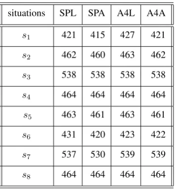
It can be observed in Table 4 that L-values are higher than corresponding A-values. In general, SP is slightly better thanA4, but not always

e.g. A4L(s8) = 423 < SP L(s8) = 431. On the basis of other similar experiments, it looks like that advantages of

SP may be more prominent but only for A-testing. Espe-cially for KB with more marginals and when values of all symptom variables are known. As far as ”Leave one out” method is concerned andnotwith full-sized evidence, no de-cisive conclusions can be drawn, so far. However, it seems thatSP does quite well and could be used along with other recommended methods.

7 Discussion and conclusions

Among positive features of marginal-less SP algorithm, the following ones can be mentioned :

1. The presented algorithmSP is sufficiently fast i.e. de-cisions are made within seconds.

2. SP has good discernment power when the tested case

t was included in the learning fileLand values of all symptom variables (from L ) are given as input evi-dence.

3. It is easy to add new cases (or remove old ones if considered as obsolete) to the learning file L. In marginal-based approach, it is necessary to recalculate the marginals.

4. Problems associated with selection of marginals are avoided (by definition !) and only symptom variables are necessary. In general, values of all symptom vari-ables (present in the learning fileL) should be provided as evidences, if available.

5. Testing via ”Leave one out” technique is extremely easy with a small modification in the presented code ofSP. It takes approximately the same time as testing on the all data (i.e. whenL =T). Marginal-based algorithm require for ”Leave one out” a lot of time for splitting the data file (|F |) times !) and filling the marginals for each split.

6. If an evidencev ∈Ξturns up, as input forSP, that is not present in the learning fileLi.e.

v6∈((F)j)Ξ forj= 1,2,· · · |F |

then SP recommends the diagnosis with the highest apriori probability i.e.

SP(v) = argmax

dj∈η

Pη(dj)

what sounds as one would expect.

7. If there is a valid piece of knowledge of logical nature (e.g. implications), it is possible to force it out just by repeating artificial records representing it in Lseveral times.

SP has several drawbacks as well:

1. SP can be applied only to nominal variables (i.e. not continuous, not cardinal and even not to ordinal) due to properties of the proximity metricsρ.

2. As the only testing criterion is number of wrong clas-sifications,SP, in its presented version, is not a proper choice for risk analysis.

3. With decreasing number of symptoms (evidences), dis-cernment power ofSP drops as well. (It is similar to marginal-based algorithms, as well.)

4. It is not possible to add additional knowledge about structure ofP(e.g. in form of graph models expressing conditional independence among marginals.) All is based on input data represented by the statistical fileF

(orL) only.

There are some open questions to study.

One would expect that decision quality is decreasing with increasing value k of proximity metrics ρ. It can be ob-served on testing runs. However, one would expect certain invariance or at least monotonicity in recommendeddopt. In

general, it does not always happen and recommended dopt

(9)

Table 3.Different testing situations

situations marginals∩variables active variables active space

s1 {m1, m2, m3} ∩ {ξ1−ξ33} ξ25, ξ26, ξ27, ξ32, ξ33 32

s2 {m1, m3} ∩ {ξ1−ξ33} ξ25, ξ27, ξ33 8

s3 {m2} ∩ {ξ1−ξ33} ξ26, ξ33 4

s4 {m1} ∩ {ξ1−ξ33} ξ25, ξ33 4

s5 {m3} ∩ {ξ1−ξ33} ξ27, ξ33 4

s6 {m2, m3} ∩ {ξ1−ξ33} ξ26, ξ27, ξ32, ξ33 16

s7 {m1, m2, m3} ∩ {ξ1−ξ32} ξ25, ξ26, ξ27, ξ32 16

[image:9.595.74.252.332.525.2]

s8 {m1, m2, m3} ∩ {ξ33} ξ33 2

Table 4.Comparing wrong classifications for SP and A4

situations SPL SPA A4L A4A

s1 421 415 427 421

s2 462 460 463 462

s3 538 538 538 538

s4 464 464 464 464

s5 463 461 463 461

s6 431 420 423 422

s7 537 530 539 539

s8 464 464 464 464

allsymptom variableswere supposed as equally informative. And if it would be effective, how to implement it in the exist-ing realization of the SP? Another topic that would deserve a deeper investigation into is behaviour of SP for small sets of disclosed symptom variables (so calledaperture) used for definingevidence. Though the improvement in decision qual-ity (with respect to alternative approaches) may be only sev-eral percentage points, it would be interesting to find if, on average, SP is a reliable tool for decision-making even in this situation.

To summarize, with respect to above mentioned argu-ments, SP can be recommended for decision-making on nominal symptom variables and when a sufficient learning data file is available. It may serve as an alternative to well established marginal-based algorithms for decision-making under uncertainty.It has sound basic philosophy (”Patients with similar symptoms should have a similar diagnosis”) and it is theoretically well founded (conditioning on equivalence classes induced by proximity metricsρand direct link to the optimal solution represented by formula 1). According to

simulations (described in section 6) on a realistic study case (mentioned in section 5), it does quite well and it does not re-quire sophisticated suppositions (like maximal entropy prin-ciple or Markovian blanket) about structure of approximating joint distributions. The problem with marginal selection (i.e ”how many” and ”what composition” ) is circumvented in SP. Remark:The original version (entitled ”Diagnostic problem without marginals”) was published at Wupes15 Workshop at Moninec. This is the extended version of that.

Acknowledgements

I am very grateful to the anonymous referee for valuable comments and suggestions to improve legibility of the paper. My thanks belong also to R.Jirouˇsek who drew my attention to the fact that suggested metrics can be seen as an instance of Hamming distance known from coding theory.

REFERENCES

[1] P.Cheeseman: A method of computing generalized Bayesian probability values of expert systems with probabilistic back-ground, in: Proc. 6-th Joint Conf. on AI(IJCAI-83), Karlsruhe

[2] W.E. Deming, F.F Stephan: On a least square adjustment of sampled frequency table when expected marginal totals are known, Ann.Math.Stat. 11(1940), pp. 427 - 444

[3] E.T. Jaynes: On the rationale of maximum-entropy methods, Proc. of the IEEE 70 (1980), pp. 939 - 952.

[4] Terrence L.Fine: Theories of Probability: An examination of foundations, Academic Press,1973)

[5] David Kahnemann: Thinking: Fast and Slow, (2012)

(10)

[7] O. Kˇr´ıˇz: A new algorithm for decision making with proba-bilistic background, in: Transactions of the Eleventh Prague Conference on Information Theory, Statistical Decision Func-tions and Random Processes, August 27-31, 1990, Vol. B, (Academia,Prague,1992) pp 135-143

[8] O. Kˇr´ıˇz: Comparing algorithms based on marginal problem. Kybernetika, Vol 43, (2007), No.5, 633–647

[9] O. Kˇr´ıˇz: Selecting marginals for decision making based on marginal problem. WUPES’09, Vol 43, (2009), No.5, 633– 647

[10] O. Kˇr´ıˇz: Mixing marginals for decision making based on marginal problem. In: WUPES 2012, Proceedings of the 9-th Workshop on Uncertainty Processing, (T. Kroupa,J. Vej-narová ed.), Mariánské Láznˇe 2012, pp. 114–125.