Path planning algorithm for a car like robot based on cell decomposition method

PATH PLANNING ALGORITHM FOR A CAR-LIKE ROBOT BASED ON

CELL DECOMPOSITION METHOD

NURHANUM BINTI OMAR

A project report submitted in partial

Fulfillment of the requirement for the award of the Degree of Master of Electrical Engineering

Faculty of Electrical and Electronic Engineering Universiti Tun Hussein Onn Malaysia

ABSTRACT

vi

ABSTRAK

CONTENTS

CHAPTER ITEM PAGE

TITLE

DECLARATION DEDICATION

ACKNOWLEDGEMENT ABSTRACT

CONTENTS LIST OF TABLES LIST OF FIGURES LIST OF APPENDICES

CHAPTER 1 INTRODUCTION 1

1.1 Project Background 1

1.2 Problem Statements 2

1.3 Project Objectives 3

1.4 1.5

Project Scopes

Organization of Report

3 4

CHAPTER 2 LITERATURE REVIEW 5

2.1 2.2

Theories

Configuration Space (C-space)

viii 2.3 2.4 2.5 2.6 2.7 2.8 2.9

Classifications of robot path planning methods

Comparisons of path planning methods

2.4.1 Cell Decomposition 2.4.2 Roadmap methods 2.4.2.1 Visibility graph 2.4.2.2 Voronoi diagram 2.4.2.3 Probabilistic Roadmap 2.4.2.4 Rapidly Exploring Random Trees 2.4.3 Potential Field

Graph Search Algorithms

2.5.1 Breadth First Search (BFS) 2.5.2 Depth First Search (DFS) 2.5.3 Dijkstra’s Algorithm 2.5.4 A* Algorithm Path Tracking

Car-like robot motion model Bezier Curve

Description of Previous Method

8 9 10 12 13 13 14 16 17 19 19 20 21 22 23 24 25 26

CHAPTER 3 METHODOLOGY 30

3.1 Overview 30

3.2 3.3

3.4

Software Development

Environmental Modelling Based On Cell Decomposition

3.5 3.6 3.7 3.8 3.9 Path Tracking Bezier Curve

Representation Technique in Path Planning

Implementation of Cell Decomposition using Matlab Flow Chart of the Main Coding

40 42 44

45

48

CHAPTER 4 RESULTS AND ANALYSIS 50

4.1 Overview 50

4.2

4.3 4.4

Matlab Programming

4.2.1 Implementation of workspace environment

4.2.2 Initial position and target position

4.2.3 Resolution and tolerance 4.2.4 Dijkstra algorithm 4.2.5 Kinematic modeling 4.2.6 Bezier curve

4.2.7 Path length calculation 4.2.8 Computational time Graphical User Interface (GUI) Algorithm analysis

4.4.1 The effect of resolution modification to the time 4.4.2 The effect of resolution

modification to the path length 4.4.3 The effect of dimension modification to the time 4.4.4 The effect of dimension modification to the path length 4.4.5 The effect of obstacles

x

4.5

modification to the time 4.4.6 The effect of obstacles

modification to the path length Result Analysis

64

65

CHAPTER 5 DISCUSSION 68

5.1 5.2 5.3

Overview

Comparison with other methods Discussion

68 68 72

CHAPTER 6 CONCLUSION AND

RECOMMENDATION

74

6.1 6.2

Conclusion

Recommendation

74 75

REFERENCES

LIST OF TABLES

3.1 Classification for Approximate Cell Decomposition

36

3.2 Classification for Exact Cell Decomposition 38

4.1 Resolution versus computational time 58

4.2 Resolution versus path length 60

4.3 Dimension versus computational time 61

4.4 Dimension versus path length 62

4.5 Number of obstacles versus computational time

63

4.6 Number of obstacles versus path length 64

5.1 Comparison of time and path length for the same parameter setting

xii

LIST OF FIGURES

2.1 Polygonal workspace approximated from a real environment

6

2.2 Classifications of the robot path planning methods

9

2.3 Quadtree decomposition 11

2.4 The visibility graph 13

2.5 A Voronoi diagram. 14

2.6 A PRM which nodes are chosen randomly 15

2.7 Path Planning using multiple RRTs 16

2.8 Simplified potential fields 18

2.9 Breadth First Search algorithm 20

2.10 Depth First Search algorithm 21

2.11 Dijkstra’s algorithm 22

2.12 A* algorithm 23

2.13 Representation of car-like robot in a static frame S

25

2.14 Random-based planning algorithm using different scenarios

27

3.1 Project design and development for PS1 31

3.2 Project design and development for PS2 32

3.3 Path generation algorithm development 33

3.4 Testing programming using the Matlab software

34

3.6 The tracked path in blue using kinematic controller

41

3.7 A portion of Figure 3.6 is zoomed in. 42

3.8 A 2nd order (quadratic) Bezier curve with three control points

43

3.9 A 3rd order (cubic) Bezier curve with four control points

44

3.10 A scenario represented in (a) original form (b) configuration space.

45

3.11 The black rectangular shapes are the obstacles. 47 3.12 The cell decomposition using Dijkstra’s

algorithm to find the shortest path.

47

3.13 A smooth path generated using Bezier curve. 48

3.14 The flow chart of the programming. 49

4.1 Programming code used to determine the workspace environment

51

4.2 Programming code used to specify the initial position and target position

52

4.3 Programming code used to specify the resolution and tolerance

52

4.4 Programming code used to generate Dijkstra’s algorithm

53

4.5 Programming code used to generate kinematic modelling

53

4.6 Programming code used to generate Bezier curve

54

4.7 Programming code used to calculate the path length

54

4.8 Programming code used to calculate the computational time

55

4.9 GUI for path planning algorithm using cell decomposition method

55

xiv

4.11 Output display panel 56

4.12 Exploring panel 56

4.13 Resolution versus computational time 58

4.14 Difference in resolution 59

4.15 Resolution versus path length 60

4.16 Dimension versus computational time 61

4.17 Dimension versus path length 62

4.18 Number of obstacles versus computational time

63

4.19 Number of obstacles versus path length 64

4.20 Tolerance surrounding the obstacles 65

4.21 Actual location for initial position and target position

66

4.22 A smooth path generated using kinematic and Bezier curve is zoomed in.

67

5.1 Parameter setting for cell decomposition and Voronoi diagram method

69

5.2 Final path for cell decomposition and Voronoi diagram with various number of obstacles.

LIST OF APPENDICES

APPENDIX TITLE

A Gantt Chart for Master Project 1 and 2

B Matlab Programming

CHAPTER 1

INTRODUCTION

1.1 Project Background

Mobile robots are widely used in many industrial fields. Research on path planning for mobile robots is one of the most important aspects in mobile robots research. Path planning for a mobile robot is to find a collision-free route, through the robot’s environment with obstacles, from a specified start location to a desired goal destination while satisfying certain optimization criteria. Most of existing path planning methods, such as the visibility graph, the cell decomposition, and the potential field are designed with the focus on static environments, in which there are only stationary obstacles. However, in practical systems, robots usually face dynamic environments, in which both moving and stationary obstacles exist.

consumption, the planned path is naturally required to be optimal with the shortest length.

1.2 Problem Statements

The problem of planning a path for a mobile robot in a given workspace, while avoiding obstacles, has been studied for many years. The main problem in a motion of the robot is when there are many obstacles in their workspace environment. This problem faced especially when the obstacle block the robot path and cause the robot operations interrupted and stopped. Obstacles can be divided into several characteristics such as size, location, networks and roughness of the obstacles. In addition, the obstacles can also in moving or stationary condition during the robot moves. This factor actually creates a major problem to the robot.

Most of the programs installed on the robot are fixed and difficult to alter. For example, if the obstacles position changed from the original position, the robot will not be able to detect obstacles and cannot proceed due to due to obstructed by the obstacles. Thus, the user needs to take action to alter the robot program to be compatible with the changing obstacles. This certainly takes a lot of time and energy. A program that can solve the problems mentioned above need to be developed to ensure the best robot path can be constructed and thus, provides benefits to all users. Solution methods fall into three broad categories: cell decomposition, roadmap methods and artificial potential field methods. The first two approaches transform the path planning problem into a graph search problem. In particular, cell decomposition methods partition the free space into convex, non-overlapping regions, called cells, and then employed techniques, such as the Dijkstra algorithm, to search the connectivity graph for a sequence of adjacent cells from the initial point to the goal.

3

beneficial when one is primarily interested either in offline or online implementation. A multiresolution scheme can keep the size of the resulting graph search tractable so that its search can be achieved with the limited on-board computational resources, while keeping the required accuracy.

An impressive amount of research on path planning for mobile robot focuses on simple robot dynamics, either fully actuated or underactuated with differential-wheel driven structure (close to unicycle). But in this project will be focus on car-like robots for offline path planning.

1.3 Project Objectives

The objective of this project is to develop an algorithmic method for constructing a solution to the navigation problem for a car-like robot. The study is proposed as follows:

a) To carry out path planning algorithm using cell decomposition method through an environment containing obstacles bounded by simple polygons.

b) To model the cell decomposition method on a car-like robot.

c) To develop the algorithm that can reach a target position without colliding with obstacles during movement.

1.4 Project Scopes

The scopes of study are as follows:

a) Cell decomposition algorithm is implemented for offline path planning.

b) The cell decomposition method is implemented on a car-like robot. c) The car-like robot is operated in an enclosed indoor and the locations

d) The coordinates of starting point and target point are known beforehand.

e) The obstacles are assumed to be in rectangular form, with random sizes and locations.

f) The algorithm can distinguish collision avoidance with stationary obstacles.

g) A car-like robot treated as a single point in its configuration space. h) Bezier curve will be applied in general in order to get a smooth path.

1.5 Organization of Report

CHAPTER 2

LITERATURE REVIEW

2.1 Theories

The path planning problem was originally studied extensively in robotics. It has gained more relevance in areas such as computer graphics, simulations, geographic information systems (GIS), very-large-scale integration (VLSI) design and games. Path planning still remain one of the core problem in modern robotic applications, such as the design of autonomous vehicles and perceptive system [1]. The basic path planning problem is concerned with finding a good-quality path from a source point to a destination point that does not result in collision with any obstacles. Depending on the amount of the information available about the environment, which can be completely or partially known or unknown, the approaches to path planning vary considerably. Latombe [2] provides a comprehensive survey of different path-planning algorithms.

Actually, the path planning problem is to find a path connecting some points for avoiding the collision with obstacles in a workspace.

map around the robot including the starting and target points is built. An obstacle in the workspace is represented as an approximated polygonal object. The size of a polygonal object is larger than the real size of the object. If

to that of a polygonal object, a robot can be represented as a point in the workspace map, not a polygon, because the size of every polygonal object includes the size of the robot as illustrated in Figure 2.1. This method can sim

with any accuracy. However, the workspace map is still continuous. In order to reduce the search space size, the workspace map can be transformed into various types of search spaces from the visual point of view.

(a) Real

Figure 2.1: Polygonal workspace approximated from a real environment

A search space is built by cell decomposition methods, roadmap methods or artificial potential field methods.

dimensional workspace is basically divided into a finite number of cells. The roadmap method transforms the workspace into the set of vertices and paths that enable a graph search. In the artificial potential field m

attractive force from the target point and repulsive force from the obstacles in the workspace.

.

Actually, the path planning problem is to find a path connecting some points for avoiding the collision with obstacles in a workspace. First, a two

map around the robot including the starting and target points is built. An obstacle in the workspace is represented as an approximated polygonal object. The size of a polygonal object is larger than the real size of the object. If the size of robot is added to that of a polygonal object, a robot can be represented as a point in the workspace map, not a polygon, because the size of every polygonal object includes the size of the robot as illustrated in Figure 2.1. This method can simplify the workspace map with any accuracy. However, the workspace map is still continuous. In order to reduce the search space size, the workspace map can be transformed into various types of search spaces from the visual point of view.

(a) Real workspace (b) Polygonal workspace Figure 2.1: Polygonal workspace approximated from a real environment

A search space is built by cell decomposition methods, roadmap methods or artificial potential field methods. In the cell decomposition method, a two dimensional workspace is basically divided into a finite number of cells. The roadmap method transforms the workspace into the set of vertices and paths that enable a graph search. In the artificial potential field method, a robot moves based on attractive force from the target point and repulsive force from the obstacles in the Actually, the path planning problem is to find a path connecting some points First, a two-dimensional map around the robot including the starting and target points is built. An obstacle in the workspace is represented as an approximated polygonal object. The size of a the size of robot is added to that of a polygonal object, a robot can be represented as a point in the workspace map, not a polygon, because the size of every polygonal object includes the size of plify the workspace map with any accuracy. However, the workspace map is still continuous. In order to reduce the search space size, the workspace map can be transformed into various

(b) Polygonal workspace Figure 2.1: Polygonal workspace approximated from a real environment [3].

7

2.2 Configuration Space (C-space)

In path planning for mobile robotics, the vehicle and the world through which it travels must both be represented in some manner so that plans can be evaluated in a search space. The search space represents all the possible situations that can exist. In order to plan a robot's motions when there are many degrees of freedom, a construction called a configuration space is used.

Lozano-Perez [4] has an idea to handle the first consideration of the configuration space. It suggested that instead of handling a complex geometrical representation of a robot in the Euclidean representation of the workspace, the robot can treated as a point in its configuration space.

At every point in time, a robot can have exactly one combination of its position and orientation. This unique combination is called a configuration. A configuration space (C-space) represents each possible configuration as a single point and contains all of the possible configurations of the robot. All of the physical obstacles from the robot's working space are mapped or transformed into this configuration space. This c-space is used where the combination of position and orientation is mapped into a single configuration point, because it transforms the problem from planning complex object motion to planning the motion of a point.

2.3 Classifications of robot path planning methods

The mobile robot path planning task is to find a collision free route, through an environment with obstacles, from a specified start location to a desired goal destination while satisfying certain optimization criteria. The path planning method could be classified into different kind based on different situations. Depending on the environment where the robot is located in, the path planning methods can be classified into the following two types:

i. Offline types – path planning in static environment which only contains the static obstacles in the map.

ii. Online types – path planning in a dynamic environment which has static and dynamic obstacle in the map.

Each of these two types could be further divided into two sub-groups depending on how much the robot knows about the entire information of the surrounding environment:

i. Path planning in a clearly known environment in which the robot already knows the location of the obstacles before it starts to move. The path for the robot could be the global optimised result because the entire environment is known.

9

Figure 2.2 shows the hierarchy of the classifications of the robot path planning methods.

Figure 2.2: Classifications of the robot path planning methods

However, this project only focussed on offline type which is static and known environment. In a static and known environment, the robot knows the entire information of the environment before it starts travelling. Therefore, the optimal path could be computed offline prior to the movement of the robot.

The path planning techniques for a static and known environment are relatively mature. Representative path planning methods for a clearly known static environment include the visibility graph method, Voronoi diagrams method, the grids method, the cell decomposition method and potential field method.

2.4 Comparisons of path planning methods.

There exist a large number of methods for solving the basic motion planning problem. Most methods of planning use one of three types of configuration space representation, called roadmap, cell decomposition and potential fields. Roadmaps model connections between special points, cell decomposition methods break the world into grids, and potential fields apply mathematical fields to model the world.

Path planning in known static environment

Path planning in unknown static

environment

Path planning in known dynamic environment Path Planning

Path planning in dynamic environment (online) Path planning in static

environment (offline)

Path planning in unknown dynamic

Among these three methods, cell decomposition is the one most widely used for outdoor robotics and quite attractive. It allows generation of collision-free paths, whereas visibility graph only guarantees semi-free paths. It is also practical compared to Voronoi diagram which appears more difficult to implement and it takes global knowledge into consideration, unlike local potential field.

Furthermore, the path generation of cell decomposition has a channel as an intermediate result if one exists. This yields at least two advantages:

i. The channel is an efficient way to answer the question if a collision-free path exists or not

ii. There are no restrictions on the generated path other than that it must be inside the channel (in contrast to Voronoi diagram and visibility graph where the path is immediately generated).

Hence, cell decomposition constitutes a good foundation for a path planning method. However, each of these types may be either topological or metric in nature. All the methods mentioned below in general must be discrete, except for the potential field method, which can also be implemented in a continuous state space fashion. These approaches will be briefly introduced below.

2.4.1 Cell Decomposition

Cell decomposition methods are the most studied and widely applied methods for outdoor robotics. In these methods the planning space is broken up into discrete, non-overlapping regions which are subsets of the c-space and whose union is makes up exactly the entire c-space. The result is a graph in which each cell is adjacent to other cells. The method for traversing from one cell to adjacent cells is called the connectivity graph. A planner then searches through the connectivity graph and the path generated is a sequence of cells the robot should traverse to reach the goal. The cost of traversing a cell may vary and the planner must apply a metric to determine which the optimal path is. Cell decompositions are often used to represent the physical space itself, but can also be used on a configuration space.

11

Adaptive cell decomposition is used to reduce the number of cells used in open areas (in order to waste less memory storage space and computation time) and to remove the digitization bias of the regular cell decomposition. The most common type of adaptive decomposition is a quadtree.

[image:23.595.193.451.325.477.2]

The quadtree method is another algorithm for searching the collision free path for a robot. It uses small non-overlapping grid cells to represent the entire environment. The cells usually are simple squares. There are three types of cells: empty cell, mixed cell and full cell. An empty cell is a free space, where the robot could go through in the environment. A mixed cell contains obstacles and free space. A full cell is the block of the obstacles. In a two-dimensional map, a quadtree is used to decomposition the map as shown in Figure 2.3.

Figure 2.3: Quadtree decomposition [5]

It begins by imposing a large size cell over the entire planning space. If a grid cell is partially occupied, it is sub-divided into four equal subparts, which are then reapplied to the planning space. These subparts are then subdivided again and again until each of the cells is either entirely full or entirely empty. The resulting map has grid cells of varying size and concentration, but the cell boundaries coincide very closely with the obstacle boundaries.

2.4.2 Roadmap methods

The second major types of representation for path planning are the Roadmap Methods. Roadmaps are graphs which represent how to get from one place to another. The roadmap approach to path generation consists of reducing the environmental information to a network of one-dimensional curves, called the roadmap. Once the roadmap has been constructed, a path can be calculated by connection the initial and final configurations to the network and finding a path in the roadmap.

Roadmaps provide a huge advantage over cell decompositions in the number of nodes a planner needs to search through in order to find a path. The set of nodes does not consist of all of the configurations, but a select few that are special. This makes them harder to create, but easier to manipulate and use. On the downside, roadmaps are generally difficult to update or repair as the robot gains new information, because the entire roadmap typically needs to be remade. In addition, most of the methods of creating the graph use artifacts of the map, such as corners of objects or crossroad to generate the landmarks and area boundaries, rather than things that can be sensed by the robot.

In general, roadmap methods are fast and most of them are easy to implement, but they do not provide an intrinsic way of describing the environmental information [2]. Examples of roadmap methods are the visibility graph, Voronoi diagram, free way net and silhouette graphs.

2.4.2.1 Visibility graph

13

[image:25.595.214.425.136.260.2]

curves) could be transformed into line segments (straight line) as shown in Figure 2.4.

Figure 2.4: The visibility graph [6]

Visibility graph methods are poor because the calculated paths are tangential to the obstacles and the robot will brush right up against the obstacles. In order to account for this, obstacle regions are generally grown to provide a safety margin, although this results in incompleteness and inefficiency of the planner. Another problem is that the obstacles must be clearly defined polygons. This is a problem for outdoor robots because obstacles almost always take on round or amorphous shapes.

2.4.2.2 Voronoi diagrams

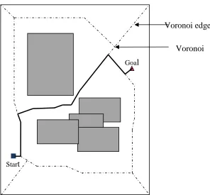
A Voronoi diagram is another popular mechanism for generating a roadmap from a c-space. It can be constructed as the robot enters a new environment. The roadmap consists of paths, or Voronoi edges, which are equidistant from all the points in the obstacle region. Voronoi diagram create roadmaps that connect the initial and goal configurations by forming paths consisting of line segments and parabolic arcs (for polygonal obstacles) that maximise the clearance between the robot and the obstacles.

Voronoi edge Voronoi

Start

[image:26.595.173.469.95.370.2]

Goal

Figure 2.5: A Voronoi diagram. The dashed lines are the set of points equidistant to obstacles. The path is shown in solid darker lines.

2.4.2.3 Probabilistic Roadmaps

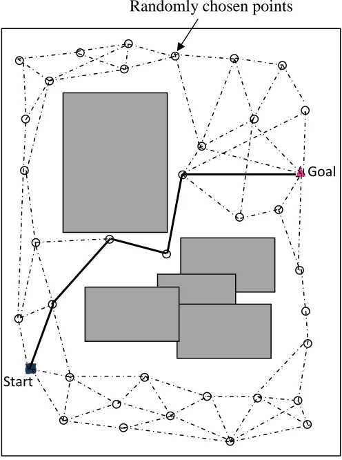
A much more recent advance in the roadmap methods is the Probabilistic Roadmap (PRM), which attempts to make planning in large or high-dimensional spaces tractable. A PRM is a discrete version of a continuous c-space which contains much fewer states than the original c-space. It is generated by randomly sampling the larger c-space and then connecting those points into a roadmap. PRMs are an improvement because most other planners, especially cell decomposition ones, tries to solve the planning problem in the entire search space. PRM methods solve in a roadmap built from a randomly chosen subset of the search space and then use a computationally inexpensive search algorithm to finish the job.

15

Randomly chosen points

Start

Goal

[image:27.595.198.446.201.534.2]

when the robot needs to plan a path between two configurations, the algorithm uses the roadmap created in the first phase to search through the waypoint nodes to find the least-cost path between the start and goal configurations. The initial graph building process is computationally expensive, however, once it has been constructed, the search is very efficient.

Figure 2.6: A PRM which nodes are chosen randomly

One problem with a standard PRM method is that it is inefficient for narrow confined spaces. Because the points which make up the roadmap are chosen at random, the chance of catching a random point in the tight space is low, and no connectivity will be established between sections of the map. Greater coverage with a greater number of nodes leads to better paths and more chance of getting through tight spots, but makes the planning more complex.

Start

Goal

means that obstacles need to be well defined and generating variable path costs is more difficult than with other methods. A third problem with PRM methods occurs when obstacles are added or removed from the map and the entire roadmap must be regenerated. Because generation of the roadmap is slow and cannot be done in real time, the planner functions poorly when the information is changing often or if the initial information is incorrect. That said, however, the roadmap construction is incremental, and can be expanded as necessary when the robot explores new terrain.

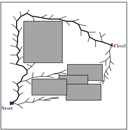
2.4.2.4 Rapidly Exploring Random Trees

[image:28.595.206.419.529.745.2]

A further variation of PRMs is the Rapidly Exploring Random Tree (RRT). Rather than randomly sampling the configuration space as a PRM does the planner begins at the start location and randomly expands a path, or tree, to cover the configuration space. The main focus is to build a roadmap in a fashion which draws the expansion of the connected paths toward the areas which have not been filled up yet. The planner pushes the search tree away from previously constructed vertices. This allows them to rapidly search large, high dimensional spaces. They are also well suited to the capture of dynamic or non-holonomic constraints, which with PRM methods have difficulty (although this capability is not critical for high level global path planning).

17

2.4.3 Potential Field

Potential Fields is the third major type of representation used in path planning. The potential field method was initially proposed by Khatib in 1986 [5] for mobile robot path planning. Potential Field methods are quite different from the previously discussed methods of planning, and have been used extensively in the past. Instead of trying to map the search space they impose a mathematical function over the entire area of robot travel.

The main idea of the method is to imagine that all obstacles can generate repulsive force to the robot, while the destination point has attractive force to the robot. Potential field method treats the robot represented as a point in configuration space as a particle under the influence of an artificial potential field whose local variations are expected to reflect the “structure” of the free space [2].

[image:30.595.129.513.76.583.2]

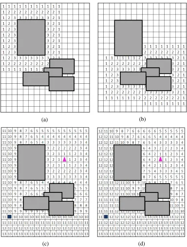
Figure 2.8: Simplified potential fields. Field produced by obstacles in (a) and (b), the field produced to create goal attraction in (c), and the sum of the fields in (d). This summed field will be used to direct the vehicle along the levels of lowest potential.

(a) (b)

19

2.5 Graph Search Algorithms

Once a method of representing the environment has been established, it is then necessary to search for the best path through that representation. These search algorithms come from wide variety of applications including general problem solving, artificial intelligence, computer networking and mechanical manipulation. In robot planning situations, the cost function (typically based on time and cost considerations) that is usually minimized is the path length. Hence, algorithms for extracting this shortest path are required to allow efficient robot navigation.

Many graph search algorithms require that every node in the graph be investigated to determine the best path. This work well when there are a small number of nodes such as in Voronoi diagram. However, when planning a path using a regular grid map over a large area, this becomes very computationally expensive. Therefore, there are many ways to traverse the graph with many adaptions.

2.5.1 Breadth First Search (BFS)

BFS is a restriction of generic search in that it explores all neighbours of a selected vertex before it goes deeper in the graph. It uses queue as its data structure to obtain the restriction. However, it does not determine which order to push the neighbours of a chosen vertex.

[image:32.595.115.543.86.280.2]

Figure 2.9: Breadth First Search algorithm [8]

2.5.2 Depth First Search (DFS)

DFS explores the graph differently than BFS. It progresses forward through the graph as much as possible, backtracking only when necessary whereas BFS first explores close vertices before going deeper to the far more vertices. It uses stack as its data structure to obtain this restriction.

The algorithm starts from a node, selects a node connected to it, then selects a node connected to this new node and so on, till no new nodes remain. Then, it backtracks to the latest node and discovers any new nodes connected to it. The data structure suitable for this purpose is a stack. Once stack is empty the algorithm ends.

DFS is an aggressive algorithm because it produces automatic ordering. DFS is written recursively as it uses stack. DFS work best for problems where there are many possible solutions, and only one of them is required. At this task, it will operate much faster than a BFS. DFS can only find the minimum length path by searching through the whole graph, rather than stopping at the first solution.

Step 1: Explore paths [A → B]

(Goal not found) [A → C]

[A → D]

Step 2: Explore paths [A →B→E](Dead end)

(Goal not found) [A →B→F](Dead end)

[A →C→G]

→ →

START A

C D

B

F E

END

[image:33.595.114.528.77.264.2]

21

Figure 2.10: Depth First Search algorithm (for this example, note that nodes D and H are never explored) [8]

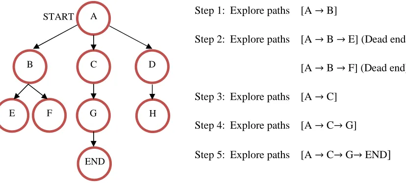
2.5.3 Dijkstra’s Algorithm

Dijkstra’s algorithm is a widely used shortest path graph searching technique. It finds the shortest path between two nodes in a graph, and in the process also extracts the minimum cost path from all nodes to the source nodes [9].

However, the ‘greedy’ nature of Dijkstra’s algorithm makes it inefficient (it must check all nodes), and hence inappropriate for searching large graphs or when limited computation time (for in real time applications) is available. Therefore, when such constraints exist, an algorithm that uses knowledge of the graph domain to improve computational efficiency is to be recommended.

Dijkstra’s algorithm solves the single-source shortest path problem for a non-negative weights graph. It finds the shortest path from an initial vertex to all the other vertices. For each vertex, the algorithm keeps track of its current distance from the starting vertex and the predecessor on the current path.

Step 1: Explore paths [A → B]

Step 2: Explore paths [A → B → E] (Dead end)

[A → B → F] (Dead end)

Step 3: Explore paths [A → C]

Step 4: Explore paths [A → C→ G]

Step 5: Explore paths [A → C→ G→ END]

START A

C D

B

F E

END

[image:34.595.103.518.81.339.2]

Figure 2.11: Dijkstra’s algorithm [8]

2.5.4 The A* Algorithm

A widely used heuristic graph searching approach is the A* algorithm, proposed by Hart, Nilsson and Raphael [9]. Unlike Dijkstra’s algorithm, this uses an ‘intelligent’ and more complicated approach to directing the graph search. It evaluates the goodness of each node, but uses a combination of the two metrics to estimates the distance to the goal: distance from the start, but also an estimated distance to the goal, like greedy search. It can also be made to be optimal if it is not made too greedy.

The goodness function for evaluating a path at each node can be expressed as follows:

f(n) = h(n) + g(n)

(2.1) Where f(n) is the goodness of the node, h(n) is the heuristic value of the node (nearness to the goal), and g(n) is the cost from the start position to the node. The algorithm will evaluate the node in the graph for which the resultant f(n) is the best. Step 1: Explore paths [OAE → END]

Path length = 11

Step 2: Explore paths [OCK → END] Path length = 12

Step 3: Explore paths [OBI → END] Path length = 8

Step 4: Explore paths [OBG → END] Path length = 7

Path is success! START 2 2 4 3 3 3 2 2 3 2 3 3 3

C L

23

The heuristic estimate, or guess, is often a calculation of what the straight line distance to the goal would be if there were no obstacles.

f(n) = Estimate of the cost of shortest solution path going through state n

[image:35.595.137.500.137.189.2]

f(n) = g(n) + h(n)

Figure 2.12: A* algorithm [8]

A* has some very good properties, which is why the algorithm is very commonly used in mobile robotics. Firstly, it will be complete provided that h(n) does not underestimate how close the node is to the goal. Secondly, it is optimal in that it will provide the fastest search of any other shortest path algorithm which uses the same heuristic.

2.6 Path Tracking

Path with piece-wise linear segments is not suitable for car-like robot with physical constraints as it leads to an abrupt change in the robot path’s direction from one segment to the next segment of the path. This path might lead to collisions with the surrounding obstacles if the robot were to traverse the path and is thus unsafe. One of the approaches to cope with this issue is to use path tracker to eliminate the need of using path smoothing technique as it allows the robot to follow the planned path safely.

The path tracking problem involves of generating a feedback control law u such that the distance to the path and orientation error tend to zero, in a mission in which a path has been planned and an autonomous vehicle has forward velocity V [10]. The following section establishes the car-like robot kinematic modeling. The the path tracking control law, which is based on car-like robot kinematic/physcal constraint is derived.

2.7 Car-like robot motion model

The car-like robots are widely used in robotics throughout the development of the path planning, obstacle avoidance and tracking systems. The model given below is based upon those described in [2].

Let Ā be a car-like robot, capable of only forward motion, modelled as a rigid rectangular body moving on a planar (two-dimensional) workspace, Ⱳ ≡ ℝ2, which is free of obstacles. Ā is supported by four wheels making point contact with the ground, while it has two fixed rear wheels and two directional (steerable) front wheels. The wheelbase (distance between front and rear wheels) is denoted by L.

For the car-like robot system, the kinematic model given by equation 2.2:

ẋ

= v cos (

θ

)

ẏ

= v sin (

θ

)

•

θ

=v tan (

ϕ

) / L

(2.2) where (x, y) are the Cartesian coordinates in a fixed frame (S) of the reference point Pm, located at mid-distance of the actuated wheels, angle θ characterizes the robot’s

77

REFERENCES

[1] P. Bhattacharya and M. L. Gavrilova, "Roadmap-Based Path Planning using the Voronoi Diagram for a Clearance-Based Shortest Path," pp. 58-66, June 2008. [2] Latombe and Jean-Claude, Robot Motion Planning, Norwell, MA: Kluwer

Academic Publishers, 1991.

[3] T. Fukuda and N. Kubota, "Trajectory and Path Planning," Control Systems, Robotics and Automation, vol. XXII.

[4] T. Lozano-Perez and M. A.Wesley, "An Algorithm for Planning Collision-Free Paths Among Polyhedral Obstacles," Communications of the ACM, vol. 22, no. 10, pp. 560-570, 1979.

[5] H. Miao, "Robot Path Planning in Dynamic Environments using a Simulated Annealing Based Approach," March 2009.

[6] N. H.Sleumer and N. Tschichold-Girman, "Exact Cell Decomposition of Arrangements used for Path Planning in Robotics," Swiss Federal Institute of Technology, Zurich, Switzerland, 1999.

[7] D. Glavaski, M. Volf and M. Bonkovic, "Mobile Robot Path Planning using Exact Cell Decomposition and Potential Field Methods," WSEAS TRANSACTIONS on CIRCUITS and SYSTEMS, vol. 8, no. 9, pp. 789-800,

[8] J.Giesbrecht and D. R. Canada, "Global Path Planning for Unmanned Ground Vehicles," Technical Memorandum DRDC Suffield TM2004-272, Canada, 2004.

[9] M. J. Barton, "Controller Development and Implementation for Path Planning and Following in an Autonomous Urban Vehicle," The University of Sydney, Sydney, 2001.

[10] R. Omar and D.-W. Gu, "Visibility Line based methodsfor UAV path planning," in Proceedings of the International Conference on Control, Automation and Systems (ICCAS-SICE), 2010.

[11] N. Ghita and M. Kloetzer, "Cell Decomposition-Based Strategy for Planning and Controlling a Car-like robot," in 14th International Conference on System Theory and Control, 2010.

[12] F. Zhou, B. Song and G. Tian, "Bezier Curve based Smooth Path Planning for Mobile Robot," Journal of Information & Computational Science , vol. 8, no. 12, pp. 2441-2450, 2011.

[13] Christian Scheurer & Uwe E. Zimmermann, "Path Planning Method for Palletizing Tasks using Workspace Cell Decomposition," ICRA Communications, 2011.

[14] F. Lingelbach, "Path Planning using Probabilistc Cell Decomposition," in Proceedings of the 2004 IEEE International Conference on Robotics &

Automation, New Orleans, LA, April 2004.

[15] R. Chatila, "Path planning and environment learning in a mobile robot system," in European Conference on Artificial Intelligence, 1982.

79

[17] F. Lingelbach, Path Planning using Probabilistic Cell Decomposition, Stockholm, Sweden: KTH Publisher, 2005.

[18] R. Johansson, "Intelligent Motion Planning for a Multi-Robot System," Royal Institute of Technology, Stockholm, Sweden, 2000.