Decreasing Value of Mechanical Stress in a
Semiconductor Heterostructure by Using Modified
Materials
E.A. Bulaeva
1, E.L. Pankratov
2,*1Nizhny Novgorod State University of Architecture and Civil Engineering, 65 Il'insky Street, Nizhny Novgorod, 603950, Russia
2Nizhny Novgorod State University, 23 Gagarin Avenue, Nizhny Novgorod, 603950, Russia Corresponding Author: [email protected]
Copyright © 2013 Horizon Research Publishing All rights reserved.
Abstract
In this paper we presented an approach to model and results of modeling of relaxation of mechanical stress in a heterostructure with porous epitaxial layer. We also presented an approach to model and result of modeling of modification of the porosity under influence of the mechanical stress. Due to the analysis of relaxation of mechanical stress and modification of porosity we obtain, that porosity of epitaxial layer leads to decreasing of value of mechanical stress in heterostructure. At the same time density of the epitaxial layer increases under influence of mechanical stress.Keywords
Semiconductor Heterostructure, Porous Layer, Decreasing of Mechanical Stress, Increasing of Density of Porous LayerPACS Numbers:
66.30.Lw, 62.20.Fe, 81.20.-n, 02.30.Jr, 02.30.Rz1. Introduction
At the present time manufacturing of semiconductor devices usually based on using semiconductor heterostructures (SH) [1-4]. Lattice spacing assumes different values in different layers of SH. Due to the difference one can obtain mechanical stress in SH. To decrease the stress it could be used materials with as small as possible difference of lattice spacing. The second way to decrease the stress is using buffer layers for gradually decreasing of difference between lattice spacing in main layers of the SH. Framework the paper we consider alternative approach to decrease the mechanical stress in SH. The approach based on using porous layers in SH. At the same time we obtain decreasing of total volume of porous. We also introduce analytical approach to model relaxation of mechanical stress and modification of porosity at one time. We find in recently published literature modeling of this processes independently from each other and in more particular cases. For example, the authors of Ref. [5] have been considered only final stage of modification of porosity, when porous are almost spherical. On the other hand it has been experimentally shown in Ref. [6], that pores are not always spherical during their modification. In the Ref. [7] it has been considered only numerical simulation of mechanical stress without accounting relaxation of mechanical stress.
2. Statement of the Problem
Figure 1. Semiconductor heterostructure with epitaxial layer (z∈[0,a]) and substrate (z∈[a,Lz]).
3. Method of Solution
We determine spatiotemporal distribution of concentrations of vacancies by solving the following equation [7,9,10]
(1)
with the initial and boundary conditions
; V(0,y,z,t)=0; V(Lx,y,z,t)=0;
,
V(x,0,z,t)=0; V(x,Ly,z,t)=0; V(x,y,0,t)=0; V(x,y,Lz,t)=0,
where S1 is the surfaces of pores; S2 is the surface of external boundary of porous region; grads and divs are operators of
surficial gradient and surficial divergence; Vn is the modulus of normal velocity of movement of surface of growing or
decreasing pore [10]; τ is the specific surface energy [9]; ω=a3, a is the atomic spacing; Ω is the atomic volume; T(x,y,z,t) is
the temperature; k=1.38⋅10-23 J/K is the Boltzmann constant; is the molar volume; µ
1(x,y,z,t)=R⋅T⋅ln(V2/V1) [9], V1 и V2
is the initial and final volume of pores, R=8.31 J/(mole⋅K) is the molar gas constant; µ2(x,y,z,t)=E(z)⋅Ω⋅σij ⋅[uij(x,y,z,t)+
uji(x,y,z,t)]/2 [8]. The relation for µ2(x,y,z,t) could be transformed to the form
(2)
where σ is the Poisson coefficient; ε0=(as-aEL)/aEL is the mismatch strain, as, aEL are lattice spacings for S and EL, respectively;
K is the modulus of uniform compression; χ is the coefficient of thermal expansion; Tr is the equilibrium temperature, which
(
)
{
( )
[
(
)
]
}
( )
[
(
)
]
+
⋅
+
⋅
=
∂
∂
t
z
y
x
grad
T
k
V
T
z
D
div
t
z
y
x
V
grad
T
z
D
div
t
t
z
y
x
V
VSV
,
,
,
,
,
,
,
,
,
,
,
1
µ
( )
(
) (
)
∫
⋅
Ω
+
VS S LzS
k
T
grad
x
y
z
t
V
x
y
W
t
d
W
T
z
D
div
0
2
,
,
,
,
,
,
,
µ
(
)
(
2)
1 2 1 2 1
2
1
,
,
,
1
V
k
T
x
y
z
t
z
y
x
V
S Vtn
=
∞+
+
+
+
τ
ω
(
)
(
)
−
+
+
=
=
,
,
∞2
− − −1
0
,
,
,
1 1 12 1 2 1 2 1
z z y
y x
x
V
e
e
e
z
y
x
T
k
V
z
y
x
f
z
y
x
V
τ
ω
V
(
)
(
)
(
)
(
)
(
)
−
∂
∂
+
∂
∂
∂
∂
+
∂
∂
Ω
=
i j j
i i
j j
i
x
t
z
y
x
u
x
t
z
y
x
u
x
t
z
y
x
u
x
t
z
y
x
u
t
z
y
x
,
,
,
,
,
,
2
1
,
,
,
,
,
,
2
,
,
,
2µ
( )
( )
(
x
)
K
( ) ( ) (
z
z
[
T
x
y
z
t
)
T
]
E
( )
z
t
z
y
x
u
z
z
ij k
k ij
ij
−
−
−
∂
∂
−
+
−
ε
χ
δ
σ
δ
σ
δ
ε
0,
,
,
3
0,
,
,
0coincide (for our case) with room temperature; E(z) is the Young modulus; σij is the stress tensor;
is the deformation tensor [11]; ui, uj are the components ux(x,y,z,t), uy(x,y,z,t) and uz(x,y,z,t) of displacement vector
; xi, xj are coordinates x, y, z. Components of displacement vector could be obtained by solving of the
following equations [11]
(3)
,
where
;
ρ (z) is the density of materials; δij is the Kronecker symbol. With account of the relation the last system of equation takes the form (4)
∂
∂
+
∂
∂
=
i j j i ijx
u
x
u
u
2
1
(
x
y
z
t
)
u
,
,
,
( )
(
)
(
)
(
)
(
)
z
t
z
y
x
y
t
z
y
x
x
t
z
y
x
t
t
z
y
x
u
z
x xx xy xz∂
∂
+
∂
∂
+
∂
∂
=
∂
∂
,
,
,
,
,
,
,
,
,
,
,
,
22
σ
σ
σ
ρ
( )
(
)
(
)
(
)
(
)
z
t
z
y
x
y
t
z
y
x
x
t
z
y
x
t
t
z
y
x
u
z
y yx yy yz∂
∂
+
∂
∂
+
∂
∂
=
∂
∂
,
,
,
,
,
,
,
,
,
,
,
,
22
σ
σ
σ
ρ
( )
(
)
(
)
(
)
(
)
z
t
z
y
x
y
t
z
y
x
x
t
z
y
x
t
t
z
y
x
u
z
z zx zy zz∂
∂
+
∂
∂
+
∂
∂
=
∂
∂
,
,
,
,
,
,
,
,
,
,
,
,
22
σ
σ
σ
ρ
( )
( )
[
]
(
)
(
)
(
)
−
( ) ( )
[
−
∂
∂
−
∂
∂
+
∂
∂
+
=
r k k ij i j j iij
x
u
x
x
y
z
t
z
K
z
T
t
z
y
x
u
x
t
z
y
x
u
z
z
E
δ
χ
σ
σ
,
,
,
3
,
,
,
,
,
,
1
2
(
)
]
( )
(
)
k kij
u
x
x
y
z
t
z
K
t
z
y
x
T
∂
∂
+
−
,
,
,
δ
,
,
,
( )
(
)
( )
[
( )
( )
]
(
)
( )
[
( )
( )
]
×
+
−
+
∂
∂
+
+
=
∂
∂
z
z
E
z
K
x
t
z
y
x
u
z
z
E
z
K
t
t
z
y
x
u
z
x xσ
σ
ρ
1
3
,
,
,
1
6
5
,
,
,
2 2 2 2(
)
( )
( )
[
]
(
)
(
)
+
( )
+
[
+
( )
( )
]
×
∂
∂
+
∂
∂
+
+
∂
∂
∂
×
z
z
E
z
K
z
t
z
y
x
u
y
t
z
y
x
u
z
z
E
y
x
t
z
y
x
u
y y zσ
σ
3
1
,
,
,
,
,
,
1
2
,
,
,
2 2 2 2 2(
)
( ) ( ) (
)
x
t
z
y
x
T
z
z
K
z
x
t
z
y
x
u
z∂
∂
−
∂
∂
∂
×
2,
,
,
χ
,
,
,
( )
(
)
[
( )
( )
]
(
)
(
)
( ) (
)
×
∂
∂
−
∂
∂
∂
+
∂
∂
+
=
∂
∂
y
t
z
y
x
T
z
y
x
t
z
y
x
u
x
t
z
y
x
u
z
z
E
t
t
z
y
x
u
z
y y,
,
,
x,
,
,
,
,
,
1
2
,
,
,
2 2 2 2 2χ
σ
ρ
( )
[
( )
( )
]
(
)
(
)
(
)
[
( )
( )
]
+
+
∂
∂
+
∂
∂
+
∂
∂
+
∂
∂
+
×
z
z
E
y
t
z
y
x
u
y
t
z
y
x
u
z
t
z
y
x
u
z
z
E
z
z
K
y z yσ
σ
12
1
5
,
,
,
,
,
,
,
,
,
1
2
2 2( )}
( )
[
( )
( )
]
(
)
( )
(
)
y
x
t
z
y
x
u
z
K
z
y
t
z
y
x
u
z
z
E
z
K
z
K
y y.
Conditions for the displacement vector could be written as
;
;
;
;
;
;
;
;
.
Spatiotemporal distribution of temperature could be described by the second law of Fourier [12]
(5)
with the initial and boundary conditions
;
;
;
T(x,y,z,0)=fT(x,y,z)=Tr.
Here λ is the heat conduction coefficient. Value of the coefficient depends on materials of SH and temperature. Temperature dependence of heat conduction coefficient in most interest area could be approximated by the following function:
λ(x,y,z,T)=λass(x,y,z)[1+ µTdϕ/Tϕ(x,y,z,t)] (see, for example, [12]). c(T)=cass[1-ϑ exp(-T(x,y,z,t)/Td)] is the heat capacitance; Td
is the Debye temperature [12]. The temperature T(x,y,z,t) is approximately equal or larger, than Debye temperature Td for
most interesting for us temperature interval. In this situation one can approximately used: c(T)≈cass. p(x,y,z,t) is the volumetric
density of heat, which escapes in the SH.
First of all let us estimate spatiotemporal distribution of temperature. To make the estimation we transform the equation (5) with appropriate conditions to the following integral form
( )
(
)
(
)
(
)
(
)
(
)
×
∂
∂
∂
+
∂
∂
∂
+
∂
∂
+
∂
∂
=
∂
∂
z
y
t
z
y
x
u
z
x
t
z
y
x
u
y
t
z
y
x
u
x
t
z
y
x
u
t
t
z
y
x
u
z
z,
,
,
z,
,
,
z,
,
,
2 x,
,
,
2 y,
,
,
2 2 2 2 2 2
ρ
( )
( )
[
]
( )
( )
(
)
(
)
(
)
+
∂
∂
−
∂
∂
−
∂
∂
+
∂
∂
+
+
×
y
t
z
y
x
u
x
t
z
y
x
u
z
t
z
y
x
u
z
z
E
z
z
z
E
5
z,
,
,
x,
,
,
y,
,
,
1
6
1
1
2
σ
σ
( )
(
)
(
)
(
)
( ) ( )
(
)
z
t
z
y
x
T
z
z
K
z
t
z
y
x
u
y
t
z
y
x
u
x
t
z
y
x
u
z
K
z
x y x∂
∂
−
∂
∂
+
∂
∂
+
∂
∂
∂
∂
+
,
,
,
,
,
,
,
,
,
χ
,
,
,
(
,
,
,
)
0
0
=
∂
∂
= xx
t
z
y
x
u
(
,
,
,
)
=
0
∂
∂
=Lx
x
x
t
z
y
x
u
(
,
,
,
)
0
0
=
∂
∂
= yy
t
z
y
x
u
(
,
,
,
)
=
0
∂
∂
=Ly
y
x
t
z
y
x
u
(
,
,
,
)
0
0
=
∂
∂
= zz
t
z
y
x
u
(
,
,
,
)
=
0
∂
∂
=Lz
z
z
t
z
y
x
u
(
,
,
,
)
0
1
=
∂
∂
Sn
t
z
y
x
u
(
)
0
0
,
,
,
y
z
u
x
u
=
(
x
,
y
,
z
,
)
u
0u
∞
=
( ) (
)
div
{
grad
[
T
(
x
y
z
t
)
]
}
p
(
x
y
z
t
)
t
t
z
y
x
T
T
c
,
,
,
=
⋅
,
,
,
+
,
,
,
∂
∂
λ
(
,
,
,
)
(
,
,
,
)
0
0
=
∂
∂
=
∂
∂
== x Lx
x
x
t
z
y
x
T
x
t
z
y
x
T
(
,
,
,
)
(
,
,
,
)
0
0
=
∂
∂
=
∂
∂
== y Ly
y
y
t
z
y
x
T
y
t
z
y
x
T
(
)
(
)
0
,
,
,
,
,
,
0=
∂
∂
=
∂
∂
== z Lz
z
z
t
z
y
x
T
z
t
z
y
x
T
(
)
(
)
(
)
[
(
)
]
(
)
×
∫
+
∂
∂
+
=
t dd
z
z
y
x
T
T
z
y
x
T
z
y
x
T
t
z
y
x
T
t
z
y
x
T
01
,
,
,
,
,
,
,
,
,
,
,
,
,
,
,
φ
τ
ϕτ
µ
ϕτ
τ
( )
∫ ∫
( )
[
(
)
(
)
]
(
)
+
(
)
+
∂
∂
+
+
−
×
d
w
d
A
x
y
z
t
w
w
y
x
T
T
w
y
x
T
w
z
x t z d assass
,
,
,
1
,
,
,
,
,
,
0 0 2
τ
τ
ϕ
µ
τ
α
(6)
.
Here
,
,
,
,
,
.
We obtain solution of the Eq.(6) by the method of averaging of functional corrections [13-15]. Within the framework of the method of averaging of functional corrections the spatiotemporal distribution of temperature has been replaced by its
average value αT1=MT1/4L3Θ, . The replacement leads to the
following result
,
where
.
Here,
.
The second-order approximation of the temperature could be obtain by the following replacing T(x,y,z,t)→αT2+T1(x,y,z,t)
in the right part of the Eq.(6). The relation is presented in the Appendix. Definition of the parameter αT2=(MT2-MT1)/4L3Θ
leads to obtaining equation to calculate the parameter. The equation is presented in the Appendix.
We used the second-order approximation for qualitative analysis and to obtain some quantitative estimation. In this situation we obtain main physical dependences and in some cases we also obtain enough good exactness of quantitative results [14,15]. Farther the distribution has been amended numerically.
Furthermore let us estimate components of displacement vector. In the common case exact solution of Eq. (4) is unknown. To obtain approximate solution we used method of averaging of functional corrections [13-15]. Let us previously transform the equations of the system (4) to the following integro-differential form.
Furthermore let us determine the first-order approximations of components of the displacement vector. To make the procedure we replace the components on their average values in the right sides of Eqs.(4), i.e. uβ(x,y,z,t)→αuβ1, β=x,y,z. The
average values can be determine as
, (7)
where
. The replacement gives us possibility to obtain
,
(
)
∫ ∫
( ) (
)
[
(
)
]
(
)
−
∂
∂
∂
+
∂
−
+
t z dass
y
x
y
z
t
w
T
x
y
w
T
x
y
w
w
T
T
x
y
w
w
d
w
d
A
0 0
,
,
,
,
,
,
,
,
,
,
,
,
α
τ
ϕτ
µ
ϕτ
τ
(
)
(
)
(
)
(
)
(
)
+
+
∫
+
−
−
−
B
x
y
z
t
B
x
y
z
t
zT
+x
y
w
t
d
w
P
x
y
z
t
F
x
y
z
y
x
,
,
,
,
,
,
1
2
,
,
,
ˆ
,
,
,
,
,
0 2
ϕ
ϕ
(
)
=
t z∫ ∫
ass( ) (
)
[
(
)
+
d]
∂
(
∂
)
g
x
y
z
t
w
T
x
y
w
T
x
y
w
T
T
x
g
y
w
d
w
d
A
0 0 2
2
,
,
,
,
,
,
,
,
,
,
,
,
α
τ
ϕτ
µ
ϕτ
τ
(
)
∫ ∫
( )
(
)
∂
∂
=
d t z assh
x
y
z
t
T
w
T
x
y
h
w
d
w
d
B
0 0
2
,
,
,
,
,
,
ϕ
µ
ϕα
τ
τ
(
)
(
)
∫
=
z +T
x
y
w
d
w
f
z
y
x
F
0
2
,
,
,
,
ϕ(
)
=
∫ ∫
t z(
)
ass
d
w
d
c
w
y
x
p
t
z
y
x
P
0 0
,
,
,
,
,
,
ˆ
τ
τ
L
=
3L
xL
yL
z(
1)
11
− +
=
ϕφ
LT
d(
)
∫ ∫ ∫ ∫
=
Θ0 0 0 0
,
,
,
x y z
L L L i i
T
T
x
y
z
t
d
z
d
y
d
x
d
t
M
(
)
(
)
(
)
+
+
−
+
=
P
x
y
z
t
+z
F
x
y
z
t
z
y
x
T
TT
ˆ
,
,
,
2
,
,
,
,
,
121 1
1
ϕ
α
φ
α
ϕ(
~
~
)
(
2
)
2
2
1+
=
Θ
Θ
+
ϕ
+
α
ϕLL
F
P
z
T
=
∫ ∫ ∫
(
−
)
+(
)
x y z
L L L
T
z
z
f
x
y
z
d
z
d
y
d
x
L
F
0 0 0
2
,
,
~
ϕ(
)
(
) (
)
∫
Θ
−
∫ ∫ ∫
−
=
Θ0 0 0 0 0
,
,
,
~
L L Lx y zass
z
z
p
x
c
y
z
t
d
z
d
y
d
x
d
t
L
t
P
Θ
=
M
L
uβ1 β1
4
α
(
)
∫ ∫ ∫ ∫
=
Θ0 0 0 0
,
,
,
x y z
L L L i
i
u
x
y
z
t
d
z
d
y
d
x
d
t
M
β β,
.
Substitution of the obtained relations in the Eqs. (7) gives us possibility to obtain the parameters αuβ1. The obtained results
could be written as
, ,
,
where
.
The second-order approximations of the components of the displacement vector can be obtained by replacing of the functions uβ(x,y,z,t) on the following sums: αuβ2+uβ1(x,y,z, t), where αuβ2=(Muβ2-Muβ1)/4L3Θ. Results of the replacement and
calculations of parameters αuβ2 are moved in the Appendix, because the results are bulky.
To determine the spatiotemporal distribution of vacancies let us transform the Eq. (1) to integral form. The integral form of the Eq.(1) is presented in the Appendix.
Furthermore we used method of averaging of functional corrections to solve the equations. The first- and the second-order approximation of vacancy concentration are also is presented in the Appendix
In the following section we analyze relaxation of mechanical stress and spatiotemporal distribution of vacancies in the SH. The obtained relations give us possibility to analysed the relaxations demonstrably. Using numerical approaches gives us possibility to amend the obtained results.
4. Discussion
In this section we analyze relaxation of mechanical stress and spatiotemporal distribution of vacancies under the influence of the mechanical stress in SH. During the analysis we obtain, that for ε0>0 total volume of pores in EL decreases. At the same
time volume of mechanical stress decreases. Probably, the decreasing of volume of pores is a consequence of compression of the EL under influence of the mechanical stress. At the same time with compression of the EL the mechanical stress also decreases. Probably, the decreasing is a consequence of increasing of density of atoms of the EL. The Fig. 2 shows dependences of component uz of displacement vector on coordinate z for porous and nonporous epitaxial layers. The Fig. 3
shows dependences of vacancy concentrations on coordinate z in stressed and unstressed epitaxial layers. The Fig. 2 shows, that mechanical stress in a SH with porous epitaxial layer decreases. Reason of the decreasing is increasing of density of porous epitaxial layer. In this situation it is possible decreasing of difference between lattice spacing in layers of the considered SH. The Fig. 3 shows increasing of density of porous epitaxial layer (i.e. decreasing of total volume of pores) under influence of relaxation of mechanical stress. Possible reason of the increasing of density of the epitaxial layer is migration of interstitials under influence of mechanical stress as under external force.
(
x
y
z
t
)
[
t
G
(
x
y
z
)
G
(
x
y
z
t
)
(
x
y
z
t
)
]
u
y1,
,
,
=
α
uy1+
φ
2 y0,
,
,
∞
−
y1,
,
,
−
α
uy1Φ
y0,
,
,
(
x
y
z
t
)
[
t
G
(
x
y
z
)
G
(
x
y
z
t
)
(
x
y
z
t
)
]
u
z1,
,
,
=
α
uz1+
φ
2 z0,
,
,
∞
−
z1,
,
,
−
α
uz1Φ
z0,
,
,
( )
( )
[
]
(
) ( )
∫
−
Θ
Χ
−
∞
Χ
Θ
=
z
L z
x x
z ux
z
d
z
z
L
L
L
0 3
2 0
1
8
ρ
α
[
( )
( )
]
(
) ( )
∫
−
Θ
Χ
−
∞
Χ
Θ
=
z
L z
y y
z uy
z
d
z
z
L
L
L
0 3
2 0
1
8
ρ
α
( )
( )
[
]
(
) ( )
∫
−
Θ
Χ
−
∞
Χ
Θ
=
z
L z
z z
z uz
z
d
z
z
L
L
L
0 3
2 0
1
8
ρ
α
( )
∫
∫ ∫ ∫
(
−
) ( ) ( ) (
∂
∂
)
Θ
+
=
Θ
Χ
Θ0 0 0 0
,
,
,
1
L L Lx y z zi
i
d
z
d
y
d
x
d
t
t
z
y
x
T
z
z
K
z
L
t
β
χ
Figure 2. Normalized dependences of component uz of displacement vector on coordinate z for nonporous (curve 1) and porous (curve 2) epitaxial layers. Here are ε0=0.02, E1=0.1, E2=0.12, K1= 0.5, K2=0.6, σ1=0.15, σ2=0.17. It should be noted, that we do not consider any concrete material. We consider some
parameters to test our solution
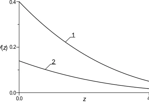
Figure. 3. Normalized dependences of vacancy concentrations on coordinate z in unstressed (curve 1) and stressed (curve 2) epitaxial layers. Here are
ε0=0.02, E1=0.1, E2=0.12, K1= 0.5, K2=0.6, σ1=0.15, σ2=0.17. It should be noted, that we do not consider any concrete material. We consider some
parameters to test our solution
5. Conclusion
In this paper we analyzed relaxation of mechanical stress in a semiconductor heterostructure. It has been shown, that using of porous epitaxial layer gives us possibility to decrease value of mechanical stress in the structure. At the same time with decreasing of the value of the mechanical stress total volume of pores decreases under special condition. The condition has been determined in the paper.
Appendix
The second-order approximation of the temperature could be written as
z
0.0 0.2 0.4 0.6 0.8 1.0
U
z1
2
0.0 a
z
V
(
z
)
1
2
0.40.2
0.0
0.0 a
(
)
(
)
[
(
)
]
{
[
(
)
]
}
∫
+
+
+
×
+
+
=
TT
x
y
z
t
t TT
x
y
z
TT
x
y
z
T
dt
z
y
x
T
0 2 1 2 1
1 1
2
2
,
,
,
,
,
,
,
,
,
,
,
,
ϕϕ
µ
τ
α
τ
α
φ
α
(
)
( )
+
(
)
+
(
)
−
(
)
−
(
)
−
∂
∂
×
d
z
A
x
y
z
t
A
x
y
z
t
B
x
y
z
t
B
x
y
z
t
z
z
y
x
T
y x
y x
ass
,
,
,
,
,
,
,
,
,
,
,
,
,
,
,
1 1
21 21
[image:7.595.183.430.307.477.2],
where
,
Equation for calculation the parameter αT2 could be written as
,
where
,
.
The integro-differential equations for components of displacement vector
( )
{
[
(
)
]
(
)
}
(
)
+
(
)
−
∫ ∫
∂
∂
+
+
+
−
d
w
d
P
x
y
z
t
w
w
y
x
T
T
w
y
x
T
w
t z
d T
ass
,
,
,
1
,
,
,
ˆ
,
,
,
0 0
2 1
1
2
τ
τ
ϕ
µ
τ
α
α
ϕ ϕ(
)
[
]
{
[
(
)
]
}
(
)
+
(
)
−
∫ ∫
+
∂
+
∂
+
∂
∂
−
d
w
d
F
x
y
z
w
w
y
x
T
w
T
w
y
x
T
w
y
x
T
t z
d T
T
,
,
,
,
,
,
,
,
,
,
,
0 0
1 1
2 1
2
τ
τ
µ
τ
α
τ
α
ϕ ϕ(
)
[
(
)
]
∫
+
+
−
− z +T
T
x
y
w
t
d
w
0
2 1
2
1
,
,
,
2
α
ϕϕ
(
)
=
∫ ∫
t z ass( )
[
Ti+
j(
)
]
{
[
Ti+
j(
)
]
+
d}
×
j i
g
x
y
z
t
w
T
x
y
w
T
x
y
w
T
A
0 0
,
,
,
,
,
,
,
,
,
α
α
τ
α
τ
ϕµ
ϕ(
)
τ
τ
d
w
d
g
w
y
x
T
j2 2
,
,
,
∂
∂
×
(
)
∫ ∫
( )
(
)
∂
∂
=
t z iass d
i
h
x
y
z
t
T
w
T
x
y
h
w
d
w
d
B
0 0
2
,
,
,
,
,
,
ϕ
µ
ϕα
τ
τ
( )
[
(
)
]
{
[
(
)
]
}
(
)
×
∫ ∫ ∫ ∫
+
+
+
∂
∂
Θ
0 0 0 0
1 1
2 1
2
,
,
,
,
,
,
,
,
,
x y z
L L L
d T
T
ass
z
T
x
y
z
t
T
x
y
z
t
T
ϕT
x
z
y
z
t
d
z
d
y
d
x
ϕ
µ
α
α
α
(
)
∫
(
)
∫ ∫ ∫
(
)
{
[
(
)
]
(
)
}
(
)
×
∂
∂
+
+
+
−
−
Θ
−
−
Θ
×
Θ0 0 0 0
2 1
1
2
,
,
,
1
,
,
,
x y z
L L L
d T
z
z
T
x
y
z
t
T
T
x
z
y
z
t
L
t
t
d
t
α
ϕµ
ϕ
ϕ( )
∫
(
)
∫ ∫ ∫
[
(
)
]
{
[
(
)
]
}
×
∂
+
+
∂
+
−
Θ
−
×
Θ0 0 0 0
1 2 1
2
,
,
,
,
,
,
x y z
L L L
d T
T ass
z
T
t
z
y
x
T
t
z
y
x
T
t
t
d
x
d
y
d
z
d
z
ϕϕ
µ
α
α
α
(
)(
)
[
(
)
]
×
∫ ∫ ∫ ∫
+
+
−
+
+
+
−
∂
∂
×
Θ +0 0 0 0
2 1
2 21
21
1
,
,
,
2
1
~
~
~
,
,
,
L L Lx y zT y
x
z
z
d
z
d
y
d
x
d
t
P
A
A
T
x
y
z
t
L
z
t
z
y
x
T
α
ϕϕ
(
−
)
−
~
1−
~
1+
Θ
~
=
0
×
L
zz
d
z
d
y
d
x
d
t
B
xB
yF
(
)
[
(
)
]
{
[
(
)
]
}
(
)
×
∫
Θ
−
∫ ∫ ∫
+
+
+
∂
∂
=
Θ0 0 0 0 2
2
,
,
,
,
,
,
,
,
,
~
L L Lx y z jd j
Ti j
i T j
i
g
g
t
z
y
x
T
T
t
z
y
x
T
t
z
y
x
T
t
A
α
α
ϕµ
ϕ( )(
z
L
zz
)
d
z
d
y
d
x
d
t
ass
−
×
α
∫ ∫ ∫ ∫
(
) ( )
(
)
×
∂
∂
−
=
Θ0 0 0 0
2
,
,
,
~
L L Lx y zi ass
z i
h
L
z
z
T
x
h
y
z
t
d
z
d
y
d
x
B
ϕ
α
(
)
µ
ϕd
T
t
d
t
−
Θ
×
(
)
(
)
(
)
(
)
(
)
+
+
−
+
=
u
x
y
z
t
C
−−x
y
z
t
C
x
y
z
t
C
x
y
z
t
t
z
y
x
u
x x xxxyxz xyyyzz xzzzyy,
,
,
2
1
,
,
,
2
1
,
,
,
6
1
,
,
,
,
,
,
5111 1101 1101(
∞
)
−
(
∞
)
−
(
∞
)
−
(
)
+
−
t
C
−−x
y
z
t
C
x
y
z
t
C
x
y
z
t
D
x
y
z
t
xxxyxz xzzzyy
xyyyzz
xxxyxz
,
,
,
,
,
,
2
,
,
,
2
,
,
,
6
0 1100
1100 10
![Figure 1. Semiconductor heterostructure with epitaxial layer (z∈[0,a]) and substrate (z∈[a,Lz])](https://thumb-us.123doks.com/thumbv2/123dok_us/8787695.907759/2.595.61.546.90.253/figure-semiconductor-heterostructure-epitaxial-layer-z-substrate-lz.webp)