Income distribution in Romania

Munich Personal RePEc Archive

Income distribution in Romania

Molnar, Maria

Institute of National Economy - Romanian Academy

2010

Online at

https://mpra.ub.uni-muenchen.de/30062/

1

Income distribution in Romania

Maria Molnar

Abstract

The paper presents the main results of a study on income distribution during 1995-2008 years, which central concern is the measurement of income inequality and polarization in Romania. A set of indices (S80/S20, Gini, Atkinson and Theil, for inequality; Foster-Wolfson, Milanovic, Wang-Tsui, Esteban-Ray and Esteban-Gradin-Ray, for polarization), have been estimated in order to get a complex and robust evaluation of these two characteristics of the income distribution. Estimates, based on data collected by Household Budget Surveys, are showing an increase ininequality and polarization, mainly since 2000 year.

Introduction

Romania is one of the EU Member States with the highest income inequality. In 2008, the Gini coefficient estimated for the monetary income distribution in Romania (36%) was by eleven percentage points higher than the same index estimated for Czech Republic and Hungary (the lowest among EU Member States), and the income quintile share ratio (7:1) was two times higher.

The income inequality in Romania is perceived as very high by most people. Hence according to the Public Opinion Barometer Survey the greatest part of the population is thinking that the Romanian society should be an equalitarian one (Bădescu, 2003). This perception derives from the strong increase of inequality during the transition from the command to the market economy, which involves a transition from an equalitarian distribution to a distribution matching the rules and mechanisms of the market. It is a distribution marked by wider income differences partly related to the reward of hard and innovative work and its results, education, talent and risk taking, largely considered as a condition of the efficient use of the productive factors and a driving force of economic development.

However the inequality is deemed to be too high and unfair because of the deep gaps between the living conditions of the greater part of population and the visibly luxurious life of the rich. The common believe that the income and wealth distribution is unjust derives also from the notorious fact that many of the very high incomes and wealth come from activities or from capital gained in the shadow economy, from breaking the law or taking advantage of law weaknesses, and from corruption. The fast growth of the income earned by some people, while a lot of poor lack the opportunities and possibilities/capabilities to have a good employment, if any, is also disturbing. The income distribution is characterized also by large differences between the incomes earned by employers, employees or some independents and those earned by farmers or received by unemployed and most of retired people, between the income and living conditions of households in urban and rural areas, and some of these differences are widening. This has led to the idea that there is a process of social polarization, suggested also by the fact that some population categories traditionally belonging to the middle class (teachers, doctors, civil servants, etc.) have relatively low wage earnings.

The generally low living standard of households in Romania, as compared to other European countries and to the expectations related to a fast and widespread increase in welfare with the

1

transition to the market economy, worsens the feeling that the distribution is unfair, which affects the economic and social behaviour, and social cohesion as well.

The inequality and the polarization have been and remained a subject of concern for social and economic policy makers, for media and for political debate (especially during elections) as well as for social and economic researchers. Yet in Romania the income distribution has been less a subject of the economic research, and consistent evaluations of income/consumption inequality have been produced only after 1995 year, based on a new source of reliable data collected by households’ surveys. Data on inequality indicators have been published by several reports and studies on poverty produced under the aegis of World Bank, UNDP, UNICEF, and by National Anti-Poverty and Social Inclusion Commission, Ministry of Labour and National Institute of Statistics. Two inequality indicators are estimated annually by the National Institute of Statistics in the framework of social inclusion indicators. Results of the evaluation of the income polarization have not yet been published, although there were some concerns (Molnar 2005, tefanescu 2008). This paperpresents some results of a studyaiming the measurement of income inequality and polarization (Molnar, 2009), a first part of an ongoing research project on income distribution in Romania.

The paper has four parts. First part focuses onsome methodological issues of income inequality and polarization measurement. The results of the estimation of the main inequality and polarization indices during 1995-2008 are being presented in the second and third part, respectively. The forth part contains an evaluation of the impact of the income redistribution on inequality and polarization.

1. Methodological issues 1.1. The data

The income concept that is used in my study is the equalized disposable income of households,

which is the best income proxy of the household’s welfare. The disposable income is estimated on the basis of information collected by the household budget surveys2. Unlike the income concept applied in Eurostat’s current inequality estimates (the monetary disposable income), the disposable income that I use takes into account the income in kind. As the consumption from own resources is an important part of Romanian households’ consumption, especially of households with low monetary income, not considering this income component is leading to the overestimation of the income inequality and polarization in Romania.

Of course, using a disposable income estimated by including income in kind, the measures come close to the actual extent of inequality and polarization. In case of Romanian income distribution, that means a lower inequality and polarization than estimated on the basis of monetary income3. However, it must be mentioned that an another important income in kind, the imputed rent is not taken into account, and it is likely that the inequality measures show a lower inequality, as almost all households are living in the accommodation they own and the

2

According to these surveys methodology the disposable income of each household is a sum of the income earned

by the household’s members or by the household as a whole from all sources (the total gross income), less payments

made by the households in redistribution (taxes and social contributions). The total gross income comprises is

estimated by adding monetary incomes (wage earnings, cash income from agricultural and non agricultural

independent activities, income from property, cash social benefits, transfers from other households and other cash

incomes) and incomes in kind (the value of some benefits in kind received by employees and persons under the

coverage of the social protection schemes, and the value of the agricultural food and non-food products consumed by household from own resources, mainly from own production, from private transfers in kind or from payment in kind for work in other households’ production).

3 _{In 2008, for example, the difference between the Gini coefficients estimated on the basis of disposable income,}

3 households with higher income generally have better accommodations. The same lessening effect on inequality and polarization measures derives from the fact that, due to the seasonality of agricultural production and the survey sample design, the expenditure made for the household production cannot be subtracted from the income earned from this source by each household. The households disposable incomes are equalized by using an equivalence scale applied in the measurement of absolute poverty in Romania. The number of adult equivalent units of a household (AE) is determined according to the formula , where A and C symbolize the number of adult persons and children in the household composition, and whose parameters, α = 0.5 and θ = 0.9, have been estimated on the basis of households’ consumption expenditure (World Bank 2003).

To observe the evolution of the income inequality and polarization during a long period the statistical information provided by two household surveys have to be used, namely the Households Integrated Survey (HIS) and the Households Budget Survey (HBS), conducted by the National Institute of Statistics (NIS) during 1995-2000 and since 2001, respectively. The income module of two surveys wasn’t modified, so the estimates of inequality indicators are comparable since 1995 year. This makes possible to observe the inequality and polarization under different economic circumstances. Unfortunately, no comparable data on the disposable income before 1995 are available, so that an analysis of the inequality and polarization throughout the period of transition to the market economy cannot be made. A family budget survey has been conducted yearly by NIS before 1995 year too, but due to methodological differences, one can hardly estimate comparable inequality and polarization indices for the entire transition period. Yet, there can be done no assessment of income distribution in the current economic crisis either.

1.2. The indices

The paper deals with the evaluation of two aspects of income inequality: the overall inequality

and the between-group income inequality.

To assess the overall inequality of Romanian households’ income, that is the inequality of

individual incomes, I used a set of indices: six quantile based indices (quintile and decile ratios, the quintile and decile share ratios, and the normalised quintile and decile absolute gaps)4, three indices derived from the common measures of variation (the Kuznets/Robin Hood index, Éltető -Frigyes indices and the variance of logarithms), the Gini coefficient, the Theil index and four Atkinson indices. I estimated several indices in order to get a refined evaluation of the inequality and polarization and their evolution in Romania and to prove the robustness of the conclusions based on the estimates, since each index has its advantages and weaknesses, and due to the fact that different indices are sensitive to changes in different parts of the income distribution (bottom, middle or top). The evaluation of between-group inequality aims mainly to evidence

the influence of some factors related to households’ characteristics. It is measured using the mean incomes of the households groups. Besides the ratio of each group’s mean equalised disposable income to the overall mean income, a statistical indicator generally used in such evaluations, I estimated also the inter-group Theil and Gini indices.

4

The quintile and decile ratios are the ratios of the top to the bottom income quintiles (Q4/Q1) and deciles (D9/D1),

respectively, while the normalised quintile and decile absolute gap is the difference between the top and bottom

quintiles (Q4 - Q1) and deciles (D9 - D1), respectively, normalised by dividing to the median (Me). The quintile share

To evaluate the polarization of the household incomes in Romania, I used several indices

derived from both of the two approaches to defining and measuring the polarization largely present in the economic literature since 1990 years. Three of the indices used in my study belong to the first approach centered on bipolarization: the Foster-Wolfson index, the Wang-Tsui index

and the index proposed by Milanovič. I estimated also the population and the income shares of the ”middle class” (the proportion of population whose income are lying in the range of 85-130%, 75-150% or 50-200% of the median income, and its share in the total income) that are also indicators related to this polarization concept. The Esteban-Ray and Esteban-Gradin-Ray indices, for bipolarization, as well as the Esteban-Ray index and the index proposed by Gradin for group polarization, are the indices derived from the second approach, based on the

relationship between polarization and conflict/social tension, which I estimated.

To assess the contribution of the redistribution in mitigating income inequality and polarization

I used the difference between the Gini coefficients (and Foster-Wolfson indices, respectively), estimated for the total gross income before social transfers (pensions included in social transfers), for the total gross income before social transfers (pensions excluded from social transfers) and for the total gross income after social transfers, in addition to that estimated for the disposable income. The total effect of the redistribution is estimated by the difference between the inequality and polarization indices of total gross income before social transfers (pensions included in social transfers) and those of disposable income, that is the difference between the inequality and polarization of income a household would dispose in the hypothetical situation of the absence of the redistribution and that of income it really disposes.

Finally, I must mention that while the most indices have been estimated based on microdata, the Wang-Tsui, Milanovic, Esteban-Ray and Esteban-Gradin-Ray indices have been estimated by using data on income percentiles or income percentile shares.

2. Inequality indices in Romania

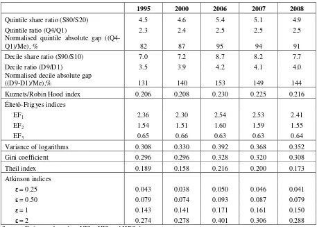
To observe changes in income inequality in the period 1995-2008, I estimated the inequality indices for five years: 1995, 2000, 2006, 2007 and 2008. It is a period marked by a severe decline, followed by a strong increase of households’ income. Due to the economic downward and the high inflation that occurred in the second half of the 1990 years, the mean equalized disposable income of Romanian households was by 25% lower in 2000 compared to 1995 year, making worse the living standard already low during the command economy and further decreased in the first years of the transition to the market economy. The decrease of the mean income was driven by falling of wage earnings and state insurance pensions (by 11% and 18%, respectively), and by the drop of the number of wage earners (from 6.2 million in 1995 to 4.6 million in 2000, along with the increase of pensioners (from 5.2 to 6.2 million), of people employed in agriculture, mainly in the subsistence one, and by the persistence of high unemployment (one million of unemployed).

Since 2001 the income increased year by year, so that in 2008 the mean income was twice that of the 2000 year’s. During 2001-2008 the average annual growth rate of the households’ income was of 9%, but in 2007 and 2008 the income increased more: by 13% and 18%, respectively. In 2008, the average wage earnings, state insurance pensions and farmer pensions were over two, two and a half and five times, respectively, higher than in 2000.

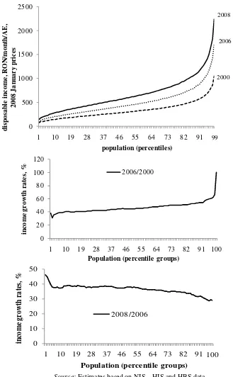
Along with that dynamic evolution of the income, the overall income inequality increased also:

5 growth of pensions5. So, while the incomes grew along the entire distribution (Figure 1) and the mean income increased by 52%, the income of the bottom 20% and 10% of the population increased only by 39% and 38%, respectively, and those of the top 20% and 10% of the population increased by 62% and 68%, respectively (Annex 1).

Table 1. Main inequality indices in Romania

1995 2000 2006 2007 2008

Quintile share ratio (S80/S20) 4.5 4.6 5.4 5.1 4.9

Quintile ratio (Q4/Q1) 2.3 2.4 2.5 2.5 2.5

Normalised quintile absolute gap

((Q4-Q1)/Me), % 82 87 95 94 91

Decile share ratio (S90/S10) 7.0 7.2 8.7 8.2 7.7

Decile ratio (D9/D1) 3.5 3.9 4.2 4.1 4.0

Normalised decile absolute gap

((D9-D1)/Me),% 131 140 153 149 144

Kuznets/Robin Hood index 0.206 0.208 0.230 0.225 0.216

Éltetö-Frigyes indices

EF1 2.36 2.30 2.54 2.53 2.41

EF2 1.54 1.51 1.60 1.59 1.55

EF3 0.65 0.66 0.63 0.63 0.64

Variance of logarithms 0.308 0.330 0.392 0.368 0.352

Gini coefficient 0.296 0.296 0.328 0.320 0.308

Theil index 0.189 0.158 0.216 0.200 0.173

Atkinson indices

ε = 0.25 0.043 0.038 0.050 0.046 0.041

ε = 0.50 0.079 0.074 0.093 0.087 0.079

ε = 1 0.143 0.141 0.171 0.161 0.150

ε = 2 0.274 0.278 0.401 0.306 0.288

Source: Estimates based on NIS – HIS and HBSdata

The faster income growth recorded in the years 2007 and 2008 has been accompanied by a reversed inequality trend: the inequality narrowed, especially in 2008, as the low incomes increased faster than the high incomes The incomes of first four quintile groups grew by 39%, 38%, 37% and 36%, respectively, while those of the top quintile group increased only by 27% (Annex 1).

The raise of the guaranteed minimum wage and of pensions, mainly due to the fact that 2007 and 2008 were election years, has been the major determinant of the decrease in income inequality. The minimum wage has been raised from 330 RON monthly, in 2006, to 390 RON, in 2007, and to 500 and 540 RON, respectively, in the first nine and the last three months of 2008 year. The average monthly state insurance and farmer pensions have increased from 311 and 117 RON, respectively, in 2006 to 523 and 159 RON in 2007 and to 593 and 253 RON in 2008. Thus the real pension increased by 23% in 2007 and 34% in 2008, while the real wage earnings increased by 15% and 14%, respectively. The monthly child allowance has been raised also from 25 RON, in 2006 and 2007, to 40 RON in 2008.

5 _{During 2001-2006, the real net wage earnings and the real state social insurance pension increased by 64% and}

However, the number of wage earners remained low, near that of 2000 year6 and the numberof pensioners and farmers was still relatively high. The gap between pensions and income from agriculture, on the one hand, and wage earnings, income from property and earnings from some independent activities, on the other hand, was large, and the distributions of earnings and of pensions have widened. Thus there were many factors that are determining a still high level of inequality in 2008.

Figure 1. Pen’s “ parade of dwarfs...” in 2000, 2006 and 2008 years

and the income growth curves

0 500 1000 1500 2000 2500

1 10 19 28 37 46 55 64 73 82 91

d is p o sa b le i n c o m e , R O N /m o n th /A E , 2 0 0 8 J a n u a r y p r ic e s population (percentiles) 2008 2006 2000 99 0 20 40 60 80 100 120

1 10 19 28 37 46 55 64 73 82 91 100

in c o m e g r o w th r a te s, %

Population (percentile groups) 2006/2000 0 10 20 30 40 50

1 10 19 28 37 46 55 64 73 82 91

in co m e g ro w th r a te s, %

Population (percentile groups) 2008/2006

100

Source: Estimates based on NIS – HIS and HBSdata

6

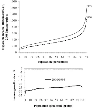
7 The estimates of the indices didn’t show an unambiguous tendency of income inequality between 1995 and 2000 years. The quantile based indices, the variance of logarithms and Atkinson (ε=2) index are showing a slight increase in inequality, the Theil index, the Éltetö-Frigyes indices and Atkinson (ε=0.25 and ε=0.5) indices are proving a decrease, while according to the Gini coefficient, the Kuznets/Robin Hood index and Atkinson (ε=1) index the inequality didn’t changed during this period. These differences related to the changes in inequality derive from the design of income falling along the distribution, due to the larger decrease in the lower part of the distribution and to an important drop in the top income (Annex 1). The income of the first and the ninth decile groups decreased by 29% and 23%, respectively; those of the tenth group fell by 28%.

Figure 2. Pen’s “ parade of dwarfs...” in 1995 and 2000 years and the income growth curve

0 200 400 600 800 1000 1200 1400 1600

1 10 19 28 37 46 55 64 73 82 91

d is p o sa b le i n c o m e , R O N /m o n th /A E , 2 0 0 8 J a n u a r y p r ic e s Population (percentiles) 1995 2000 99 -35 -30 -25 -20 -15 -10 -5 0

1 10 19 28 37 46 55 64 73 82 91

in c o m e g r o w th r a te s, %

Population (percentile groups) 2000/1995

Source: Estimates based on NIS – HBSdata

been corrected until 2000), and therefore it is likely that the 1995 year’s inequality indices are showing a higher inequality than the real one. Thus an increase in income inequality can be considered during this period also. Another reason of thinking about increasing in inequality is the high sensitivity of Romanian society to changes at the bottom of the distribution, as a large decrease in the income of poor is very painful due to the severe constraints in meeting their basic needs.

According to some evaluations based on information provided by the old Family Budget Survey, during the first years of transition to the market economy (1990-1994) there was a larger increase in inequality. It was a period characterized by strong economic decline and high inflation, the severe fall in employment, especially in salaried employment, the explosion of unemployment and the movement of the mass of workers displaced from many dismantled industrial units to the subsistence agricultural activities or to the pension system, as well as by a dramatic erosion of

wage earnings and pensions’ purchasing power. The number of wage earners fell from 8.2 million in 1990 to 6.2 million in 1995, the number of state insurance and farmer pensioners

rose from 3.7 to 5.3 million, the unemployed rose to one million until 1995, while population employed in agriculture rose to 3.2 million. The average wage earnings and the average state insurance pension fell by 34% and 39%, respectively. Along with this increase in the number of low income earners and the drop of wages and pensions there was a widening of earnings’ distribution, as a result of differences in the pace of the fall in real earnings, namely of differences in the pace of nominal earnings growth due to different bargaining power. According to the Gini coefficients estimated on the basis of wage earnings statistics, the gross earnings inequality almost doubled between 1989 (0.155) and 1995 (0.287), while Gini coefficients estimated for disposable income per household, on the basis of the old Family Budget Survey, increased from 0.237 in 1989 to 0.264 in 1994, and those estimated by B. Milanovic for the households’ gross income per capita increased from 0.233 to 0.286 during the same period (UNU/WIDER).

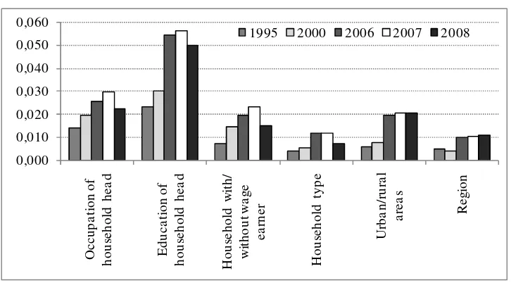
Between-group income inequality increased also. During these periods of falling and growing

incomes, some population groups lost more or earned less than others, therefore the income gaps between different categories of households have increased between 1995 and 2008.

Figure 3. Between-group Theil indices, by main household characteristics

0,000 0,010 0,020 0,030 0,040 0,050 0,060 O cc up at io n of ho us eh ol d h ea d E du ca tio n of ho us eh ol d h ea d H ou se ho ld w ith / w ith ou t w ag e ea rn er H ou se ho ld t yp e U rb an /r ur al ar ea s R eg io n

1995 2000 2006 2007 2008

Source: Estimates based on NIS – HBSdata

9 residence are also important, as well as those related to the age and gender of individuals or of households’ head. The estimates of the groups’ mean incomes ratios to the overall mean and the between-group Gini and Theil indices (Annex 3) show an increasing tendency of the intergroup income inequality during 1995-2007 years, and its decrease in 2008, except for grouping by residence areas and region.

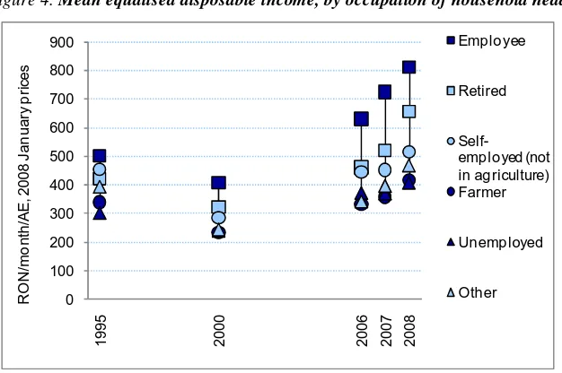
Regarding to income differences by occupation7 of household head, one can expect that

households headed by persons in employment have higher income than those headed by unemployed or inactive persons, since the amount of income received by a household depends on the position of its members in the labour market. However, according to Household Budget Survey, in Romania only the mean incomes of households whose reference person is employee (wage earner)8 exceed the overall mean. The farmer households have one of the lowest incomes, close to the incomes of the unemployed headed households. In 2008, the mean incomes of these two household categories were by 39% and 40%, respectively, below the overall mean, and two times lower than the income of households headed by wage earners. In time, due to the quick increase of wage earnings, the income gap between the first two and the last household categories widened. The same tendency has been recorded by the gap between the mean incomes of households whose reference person is a non-agricultural self-employed or an inactive (other than retired) and those of employee headed households. Although the pensions are much lower than the wage earnings, the mean equalised income of households headed by retired is not too far from that of employees’ households, due to the fact that the size of the retired headed households is usually smaller and because a part of them are mixed households, including employees. However, the gap between their mean income and that of employees’ households increased. Only in 2008 this trend has reversed due to the increase in the pension level; increase that led to a substantial drop of between these groups income inequality.

Figure 4. Mean equalised disposable income, by occupation of household head

0 100 200 300 400 500 600 700 800 900 1 9 9 5 2 0 0 0 2 0 0 6 2 0 0 7 2 0 0 8 R O N /m o n th /A E , 2 0 0 8 J a n u a ry p ri ce s Employee Retired Self-employed (not in agriculture) Farmer Unemployed Other

Source: Estimates based on NIS – HIS and HBSdata

In general, households with at least one employee (wage earner) or employer in their composition have higher incomes than those in which these categories of active persons are missing. In 2008, the mean equalized disposable income of the first household group was by 50% higher than that of the second group, and the gap was higher during 2006-2008 compared with 1995 and 2000 years.

7

Wage earner, employer, self-employed in non-agricultural activities, farmer, unemployed, retired, other.

8 _{In general, households headed by employers have the highest income levels, but statistical data on that household’s}

According to between-group Theil indices, in 2008, 13% of the overall income inequality has been related to living in households headed by persons with different occupations and the impact of this factor doubled between 1995 (8%) and 2007 (15%). The influence of living in households with or without wage earners has also increased (Annex 3).

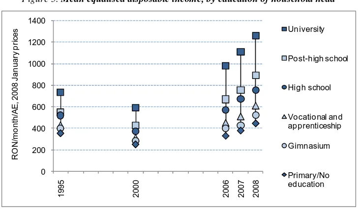
The differences related to the education are the highest, since the possibility to find a well paid

job, to perform an efficient independent activity or to start a successful business, as well as the income from work and the pension are depending to the educational attainment to a large extent. In 2008, the mean income of households headed by a person with university education was 2.8 times higher than that of households which household head has only primary or no education, and the gap increased from 2.1, in 1995, and 2.3, in 2000, to 3.0, in 2006, due to the faster income growth in case of households with the highest educational endowment. The between-group Theil indices, the highest as compared to those related to other characteristics, is showing also a large increase, from 0.023, in 1995, to 0.056 and 0.050, respectively, in 2007 and 2008. The education has the largest impact on inequality: in 2008 the education caused 29% of the total income inequality, more than twice the extent of its impact recorded in 1995 year.

Figure 5. Mean equalised disposable income, by education of household head

0 200 400 600 800 1000 1200 1400

1

9

9

5

2

0

0

0

2

0

0

6

2

0

0

7

2

0

0

8

R

O

N

/m

o

n

th

/A

E

, 2

0

0

8

J

a

n

u

a

ry

p

ri

c

e

s University

Post-high school

High school

Vocational and apprenticeship

Gimnasium

Primary/No education

Source: Estimates based on NIS – HIS and HBSdata

The household type is also an important differentiating factor of households’ equalized incomes.

11 Living in urban areas seems to be an advantage as compared to having the residence in rural areas, since the income of urban households is considerably higher than those of rural ones: by

52% on average, in 2008. Mainly the differences in occupation of the population living in urban and rural areas are leading to this income gap, namely the fact that farmer households and retired in the farmers’ pension system (which pensions were extremely low until the setting up of the social minimum pension, in 2009) are living in rural areas, while most wage earners are working and living in urban areas. Likewise, a great proportion of single elderly (mainly single old women), of households with three or more children and multigenerational households of three or more adults with dependent children are living in rural areas, as well as most low educated people. As a matter of fact, the underdevelopment of the agriculture, of the rural economy in general, the persistence of the subsistence agriculture and the lack of opportunity to get salaried employment and to attain the required education to cope with the new economic environment are the major determinants of low incomes in rural areas. Living in urban or rural areas explains more than a tenth of income inequality (12% in 2008).

The determinants of income inequality by region are the same, as the income differences

between the eight regions are mostly related by the population share of urban/rural areas. The highest income level is recorded in the region of capital city, Bucharest, and the lowest in North-East region. In 2008, the disposable income of households living in the Bucharest region exceeded those of households in North-East region by 65%, more than in 1995 and 2000 years (38% and 40%, respectively). Besides there is a large gap between Bucharest region and the other regions: the income in the former are by 36% to 65% higher than in the other regions, while the gap was of 1% to 38%, in 1995, and of 14% to 40%, in 2000. It must be mentioned also that the mean incomes in all Eastern and Southern regions (North-East, South-East, South and South-West) are lower than those in Western and Central regions (West, North-West and Centre).

The results of a multivariate analysis of households’ disposable income in 2008 (Annex 4)

show that the most important income differentiating factor is the education (with the largest range of the regression coefficients (0.82), followed by the occupation of household’s head (0.65), the household type (0.33), the region (0.19) and the urban/rural areas of residence (0.12). Keeping under control the other variables, the ratio of the predicted values of the income corresponding to the highest and the lowest educational attainment is 2.3:1 and the predicted value of urban households’ income is by 13% higher than that predicted for rural ones. All these factors have a stronger influence on the distribution of monetary disposable income, which is more unequal.

3. Income polarization indices in Romania

3.1. Bipolarization

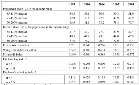
All the indicators I used to measure the income polarization show a higher degree of polarization in 2008 than in 1995. It increased in 2000 compared to 1995, and in 2006 compared to 2000, and it decreased in 2007 and in 2008 (Table 2).

means the movement of a part of the population from the middle to the extremes of distribution, by the ‘impoverishment’ of some and the ‘enrichment’ of others.

The same downward trend was recorded also by the income share of population located within the central interval, but the income ‘lost’ in the center moved towards the rich part of the distribution. The income of the population in the income range of 75-150%, for example, represented 49.5% of total income in 1995 and only 45.9% in 2008, while the income share of those whose income is higher than 150% of the median increased from 37.0% to 40.2% and the proportion of those with income less than 75% remained practically the same (13.3% and 13.8%, respectively). The increasing of the proportion of the population with income higher than 150% and lower than 75% of the median has been accompanied by an increase in the income gap between the two groups of people, from 4.1:1 in 1995 to 4.3:1 in 2008. There are two defining trends of a polarization process.

In the years 2007 and 2008, the increase of the proportion of median interval occurred on account of the top one, whose population and income share fell, unlike the one of the bottom interval which hasn’t changed significantly. It is a result of the relatively high growth of the low and medium level incomes (minimum wage and pensions, mainly), partly about the fact that those two years were electoral.

Table 2. Income bi-polarization indices

1995 2000 2006 2007 2008

Population share (%) in the income range

85-130% median 34.5 33.1 30.5 30.8 31.9

75-150% median 52.8 50.6 47.6 47.9 48.9

50-200% median 83.5 81.1 78.2 78.8 79.7

Income share (%) of the population in the income range

85-130% median 31.7 30.7 27.0 27.9 29.4

75-150% median 49.5 47.8 43.0 44.0 45.9

50-200% median 77.5 76.2 70.4 72.0 74.4

Foster-Wolfson index 0.231 0.243 0.266 0.261 0.253

Wang-Tsui index ( r = 0.5) 0.592 0.603 0.634 0.627 0.616

Milanovič index 0.349 0.360 0.383 0.378 0.372

Esteban-Ray index*

α = 1 0.206 0.208 0.230 0.225 0.216

α = 1.5 0.149 0.150 0.167 0.162 0.156

Esteban-Gradin-Ray index*

α = 1 0.116 0.120 0.133 0.129 0.124

α = 1.5 0.059 0.062 0.069 0.067 0.064

* 2 income intervals, cutt-of income level = mean

Source: Estimates based on NIS-IHS and HBS data

The increase of polarization can be seen also by comparing the first and the second curves of income polarization in the years 1995, 2000, 2006 and 2008: the highest values of the two curves are estimated for 2006 and the smallest are those estimated for 1995. The estimated values for 1995 and 2000, as those estimated for 2006 and 2008 are very close, so the first two curves, and the last two, almost overlap on the graphic representation, while the 2000 and 2006 years curves dominate visibly the 1995 and 2008 years curves, respectively (Annex 6).

13 and the decrease in 2007 and 2008. According to the Esteban-Ray index, polarization had the same increasing and decreasing tendency during 2000-2006 and in 2007-2008, respectively, but there was no change in polarization in 2000 compared to 1995. During all these three periods the direction of changes in polarization measure has been related to changes in the gap between the income over and below the mean income that affect the function of alienation, while changes in the structure of the population (which affects the function of identification) had only a slight, mainly mitigating, influence. Between 1995 and 2000, there was a slight change in the structure of the population by increasing the share of population with higher income than the average, but the gap between the averages of the income higher and, respectively, lower than the overall mean has not changed, so that polarization index remained at the same level.Between 2000 and 2006, the gap between the two averages increased (from 2.3 to 2.6), which led to increased polarization, to some extent mitigated by increasing the share of population with income lower than the overall average. In 2007 and 2008, the decrease of polarization was determined by the decrease of the gap between incomes, while the increase of the population share of those with the income above the mean had a slight influence in the opposite direction, the attenuation of the decrease of polarization (Annex 7).

The Esteban-Gradin-Ray index (EGR) show a much lower degree of polarization compared with the Esteban-Ray index (ER), as the lack of identification, determined by the inequality in income within each of the two groups, is relatively large. It can be noted also, that the EGR index shows a slightly smaller increase of polarization in 2006 compared with 2000, given that the within-group inequality increased significantly. However, the decrease in within within-groups inequality, which took place in 2007 and 2008, sustained and slightly amplified the diminishing of the degree of polarization caused by the decreasing gap between the incomes.

3.2. Incomepolarization by sub-population

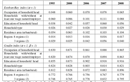
To study the extent to which a process of group income polarization arises, several Esteban-Ray (ER) and Gradin (G) indices were estimated by characteristics which have proved to be relevant for the income differences: the occupation of household head, the presence or the absence of at least one wage earner or employer in the household composition, the educational attainment of the household head, the household type, the area and the region of residence.

The Esteban-Ray indices show that the intergroup polarization increased for all the characteristics of the group until 2007 and declined in 2008, except the one related to the area of residence, which increased in 2008 too. In 2008, the highest degree of intergroup income polarization was the one generated by the urban or rural residence. The presence or absence of at least one employee (wage earner) or employer in the household composition is also an important factor of the income polarization, as it is also the occupation of the household head and his education. The type of the household has a less polarizing impact9. The polarization of the income is linked to the lowest extent to the residency in one or other of the eight regions.

However, if the Esteban-Ray index is estimated for three groups, consisting of the eastern and southern regions of the country (whose average income is less than the national average), the western and the central regions of the country (whose average income is slightly higher than the national average) and the Bucharest-Ilfov region (with income well above average), its level is more than double that estimated for the eight regions.

Thehouseholdincome is influenced by the socio-economic characteristics of the household, and that is witnessed by the gaps between the mean incomes estimated by groups formed on the basis

9 _{The much higher level of the estimated indices for groups formed according to the area of residence and the}

of these characteristics and by the intergroup Gini indices. However, these groups are not homogeneous in terms of income levels, with significant differences between the income levels of the households in each group. Also, the distributions of the income of the different groups overlap to some extent10. This considerably diminishes the sense of identification within the

group and the estimates of the correction term (ε) proposed by C. Gradin for the group polarization (which refers to the lack of identification) is relatively high compared with the between-group Esteban-Ray index. The lack of identification is higher for the regions and the group related to the presence/absence of at least one wage earner/employer in the household composition and much lower in the case of the group formed according to the education of the household head. Thedata show in general, that the lack of identification is lower in 2008 than in 1995, especially in the case of the groups formed according to the level of education and the area of residence (Annex 8).

Table 3. Group polarization indices, by households’ characteristics

1995 2000 2006 2007 2008

Esteban-Ray index (_α = 1)

Occupation of household head 0.048 0.060 0.070 0.078 0.065

Households with/without at

least one wage earner/employer 0.060 0.086 0.101 0.111 0.088

Education of household head 0.038 0.042 0.057 0.060 0.056

Household type 0.026 0.027 0.028 0.030 0.029

Residence area (urban/rural) 0.054 0.063 0.102 0.103 0.104

Region: 8 regions (1) 0.014 0.013 0.016 0.016 0.017

3 regions (2) 0.029 0.025 0.042 0.056 0.040

Gradin index (α = 1, β = 1)

Occupation of household head 0.830 0.871 0.861 0.888 0.865

Households with/without at

least one wage earner/employer 0.820 0.874 0.870 0.894 0.863

Education of household head 0.855 0.873 0.902 0.918 0.916

Household type 0.824 0.828 0.803 0.814 0.821

Residence area (urban/rural) 0.812 0.828 0.872 0.883 0.896

Region: 8 regions (1) 0.772 0.766 0.756 0.767 0.779

3 regions (2) 0.748 0.765 0.778 0.832 0.795

(1) North-East, South-East, South, South-West, West, North-West, Centre, Bucharest-Ilfov

(2) (i) North-East, South-East, South and South-West; (ii) West, North-West and Centre; (iii)Bucharest-Ilfov

Source: Estimates base on NIS-IHS and HBS data

As a result, the Gradin index of the income group polarization,estimated by subtracting from the Esteban-Ray index the error term related to the lack of identification, shows a lower increase in polarization. According to this index, the most important factor in the income polarization is the education endowment, followed by the area of residence. The region of residence has the lowest impact. The polarization by education and by the urban or rural residence has increased throughout the 1995-2008 period, given that the gap between the incomes of groups has increased and the dispersion of the income within the groups has decreased.

10 _{For example, the income of the households which have an employee as reference person vary significantly}

depending on the number of employees in the household, the level of wages earned by each of them and the presence of other active persons (self-employed or unemployed) or inactive (retired persons, children etc.) in the household composition. Also, there are many households of retired persons whose income is equal to the income of the households with employees, given that some pensions exceed the minimum wage, and the households with

15 The polarization related to the occupation of household head and to the presence/absence of employees in the household composition increased also. However, there was a decrease of it in 2006, compared to 2000, and in 2008, compared to 2007. During 2000-2006 this evolution can be explained by a large increase in the dispersion of the income within groups that occurred along with the increase in the gap between the incomes of the households grouped by the occupation of household head.In 2008, a slight increase in the lack of identification within group went along with the reducing of the gap between the income of the groups and the decrease of the between-group income polarization, due to the significant increase of the pensions.

The polarization by household type and regions was practically the same in 1995 and 2008, but lower in 2006, the year of the largest dispersion of income within the household types and regions.

4. The impact of redistribution

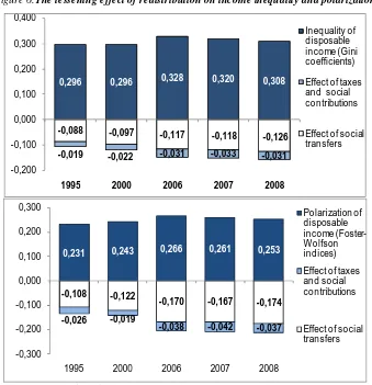
The estimates of Gini coefficients and Foster-Wolfson indices for different income concepts reveal large and growing differences between the inequality and polarization before and after redistribution, i.e. before and after social transfers and payment of taxes and contributions to social protection schemes (Annex 9).

In 2008, the Gini coefficient of the gross income before social transfers was of 0.465 and that of

the disposable income (the net income after social transfers) was of 0.308. Thus one can suppose that the redistribution led to a lessening of income inequality by 34%. Most of the total effect of redistribution was due to social transfers (80%, out of which 67% to pensions and 13% to the others social benefits).

The lessening effect of redistribution on income inequality grew during 1995-2008 period from 27% in 1995 to 31% in 2006 and to 34% in 2008 (Annex 10). The impact of both redistribution components (social transfers and taxes) increased over the entire period, except for the 2008 year’s decrease of tax contribution. The social transfers, the pensions mainly, were the leading equalizing component of redistribution over the entire period. The share of their contribution to the overall lessening effect decreased slightly from 82% in 1995 to 78% in 2007, although their share in households’ income increased. There was instead a slight increase in the share of the taxes’ contribution in the attenuation of income inequality, related mainly to the growing share of wage earnings in households’ income, given that the wage earnings are the main source of income tax revenue and of contributions to the social security systems, and to a lesser extent to changes in the tax system, except for 1995-2000 years. During that period a significant decrease of wage earnings share went along with a small increase of the equalizing effect of taxes due to an increase of social contributions rates and the setting up of the progressive taxation. The share of equalizing effect of taxes was larger in 2006 than in 2000, albeit a flat tax system has been set up in 2005. The considerable increase of wages and of their income share, as well as a loss in the pensions equalizing power (since pensions increased less than wages) led to this trend.

Obviously, the redistribution has a greater mitigating effect on the inequality between the income of households grouped by the occupation of household head, since for some households’ groups social benefits are the main income source and the taxes and social contributions are been paid mainly by the other households’ groups. In 2008, the between-group Gini coefficient estimated for the mean disposable income of these households’ groups was by 57% lower than that estimated for the gross income before social transfers. The largest part of the difference between the two Gini coefficients was also due to social transfers (70%), although the effect of taxes and social contributions was greater than on the overall inequality (30% compared with 20%).

also large, while the impact on the inequality related to education, residence areas and region is smaller(Annex 11).

Figure 6.The lessening effect of redistribution on income inequality and polarization

-0,088 -0,097 _{-0,117 -0,118}

-0,126 -0,019 _-0,022 -0,031 -0,033 _-0,031

0,296 0,296 0,328 0,320 0,308

-0,200 -0,100 0,000 0,100 0,200 0,300 0,400

1995 2000 2006 2007 2008

Inequality of disposable income (Gini coefficients) Effect of taxes and social contributions

Effect of social transfers

-0,108 -0,122

-0,170 -0,167 -0,174 -0,026 -0,019

-0,038 -0,042 -0,037

0,231 0,243 0,266 0,261 0,253

-0,300 -0,200 -0,100 0,000 0,100 0,200 0,300

1995 2000 2006 2007 2008

Polarization of disposable income (Foster-Wolfson indices) Effect of taxes and social contributions

Effect of social transfers

Source: Estimates based on NIS – HIS and HBS

The large difference, and growing, between the Foster-Wolfson indices estimated for the gross

total income without social transfers (the income of the households before redistribution) and the disposable/net income (after the redistribution) shows a large contribution of the redistribution to achieve a lower income polarization also (Annex 9).

In 2008, according to the Foster-Wolfson indices, the level of disposable income polarization was by 46% lower than the one which would have been achieved in the absence of redistribution hypothesis (0.253 and 0.465, respectively), and the difference increased compared with 1995 and 2000 (37%), 2006 (44%) and 2007 (45%). As in the case of inequality, the most important contribution to mitigating the polarization is given by the social transfers, particularly the pensions. In 2008, 82% of the impact of the redistribution was due to social benefits, of which 73% to pensions and 9% toother social benefits.Almost a fifth (18%) of the ‘diminishing’ of the polarization derived from taxation (taxes and social contributions).

17 already been established. The explanation for this development is related to the evolution of the wages and of the number of employees and to the high tax and social contribution rates on wages. The large decrease of employees’ number and in the share of wages in the households’ income during the period between 1995 and 2000 led to the decrease of the impact of taxes and social contributions on the polarization, as the increase of wages and of their share in the income have led to the increase of the impact of taxes and social contributions by 2006 and in 2007 (Annex 10).

The Esteban-Ray between-group polarization indices, estimated according to the socio-economic characteristics of the households, also show a large contribution of the income redistribution to alleviate the income polarization (Annex 11). In 2008, the extent of polarization was by 63%, 70%, 43% and 40%, respectively, lower than expected under the hypothesis of the absence of redistribution, in the case of the households’ grouping according to the occupation, the presence of at least one employee/employer in the household composition, the education level and the area of residence.

Concluding remarks

The income distribution in Romania is marked by the general low income level and a relatively high and increasing inequality. The inequality increased along the transition to the market economy, during periods of economic downturn and economic growth as well, with some trend breaks related mainly to elections. At the beginning the income inequality raised because most households suffered income losses due to high inflation and economic recession and some households became rich or very rich, by fair or unfair means. Then the growth of property income and of wage earnings and income from independent activity, related to some professions and jobs, and the persistence of a large proportion of households with low and very low incomes, related to missing qualifications and employment opportunities as well as to family burden, were the determinants of inequality widening.

Increasing inequality and particularly the large gap between the living condition of the poor and of many of those traditionally belonging to middle class and the luxurious life of the rich led to the widespread believe that there is a trend of social polarization in Romania. The results of the estimating of a set of indicators show an income polarization and its rise during the period between 1995 and 2008. All indicators show an extent of bipolarization higher in 2008 compared with 1995 and 2000, while its growth was higher between 2000 and 2006, and then declined in 2007 and 2008. The increase in the polarization and its decline over the latest two years were caused by the increase and, respectively, the decrease of the gap between high and low incomes, whereas the changes in the structure of the population had little influence and acted only in the direction of the decrease of the polarization.

As regards the group polarization of the income, the highest degrees of polarization are related to the educational level of the household head and the area of residence. They have increased throughout the period, including 2007 and 2008. The occupation of the household head and the presence/absence of at least one employee/employer in the household composition are also factors with a relatively large impact on the income polarization.

Although the social protection is low, the redistribution of income has an important contribution in levelling of income distribution, especially by social transfers. However, to diminish the present inequality and to prevent its excessive increase and further polarization the redistribution is not enough. Of course, its contribution can improve, by raising the level of social protection and by improving its efficiency, as well as by providing the necessary resources, including a better collection of taxes and social contributions, and by allocating more to social protection while sharing out the fruits of economic growth.

Policies to increase and to improve employment, especially of those experiencing difficulties in finding jobs, to reduce the employment on informal and black market and to motivate participation in work are also very important, as they can contribute to dwindle the population with low income. A proper remuneration of teachers, doctors and other medical staff, of civil servants and highly skilled experts, which are working in public institutions, and policies aimed at supporting the liberal professions can contribute to the formation and the strengthening of the middle class and to the decrease of the income polarization. The development of the agriculture, of the rural economy in general, as well as the regional development, is crucial for poverty alleviation and reducing inequality, while improving education and training, and providing equal opportunities to education is a factor that can contribute to reducing inequality and polarization in the long term.

References

Asad A., Murthi M., Yemtsov R., Murrugarra E., Dudwick N., Hamilton E., Tiongson E. (2005), ”Growth, Poverty, and Inequality. Eastern Europe and the Former Soviet Union”, The World Bank, Washington DC.

Atkinson A.B. (1970),”On the Measurement of Inequality”, Journal of Economic Theory, 2(1970): 244-63.

Bădescu, G. (2003),”Atitudini si perceptii privind inegalitatea socială în România ” (Attitudes and Perceptions on Social Inequality in Romania. Public Opinion Barometer Survey Report), Open Society Institute – international Policy Fellowships,

http://www.policy.hu/index.php?m=publication&id=21052.

Betti, G. and Lemmi A. eds. (2008), ” Advances on Income Inequality and Concentration Measures”. Routledge, London and New York.

Champernown, D.G. and Cowell F.A. (1998),” Economic inequality and income distribution”, Cambridge University Press, Cambridge.

Cowell, F.A. (2006),” Inequality: Measurement”, London School of Economics and Political Science – STICERD, Distributional Analysis Research Programme Discussion Paper (DARP), 86.

Duclos, J., Esteban, J. and Ray, D. (2004), “Polarization: Concepts, Measurements, Estimation”,

Econometrica 72 (6): 1737-1772.

Echevin, D. and Parent, A. (2002), ”Les indicateurs de polarisation et leur application en France”, Economie et Prévision 155(4): 13-30.

Esteban, J. (2002), ”Economic Polarization in the Mediterranean Basin”, Els Opuscles del CREI, 10, Center for Research in International Economics.

19 Esteban, J.M. and Ray, D. (1994), ”On the measurement of polarization”,Econometrica, 62 (4): 819-52.

Foster, J. and Wolfson, M. (1994) “Polarization and the Decline of the Middle Class: Canada and the US”, mimeo,Vanderbilt University; Journal of Economic Inequality, Published online:

19 November 2009..

Gradin, C. (1999) ”Polarization and inequality: an international comparison”, Essays on Polarization Measurement, http://decon.edu.uy/network/C/gradinc.pdf.

Gradin, C. (2000) ”Polarization by sub-population in Spain, 1973-91”, Review of Income and Wealth, 46(4): 457-474.

Ilie, S. (2004),”Inegalităţi în distribuţia veniturilor i politica socială a veniturilor (Inequalities in income distribution and income social policy)”, The Research Institute for the Quality of Life – Romanian Academy,

http://www.iccv.ro/index.php/en/download?task=view.download&cid=37

ILO (2008), ”World of work report 2008: income inequalities in the age of financial

globalization”, International Labour Organisation (International Institute for Labour Studies), Geneva.

Larionescu, M., Mărgineanu I. and Neagu G. (2006) ”Constituirea clasei mijlocii în România” (The Establishment of the Middle Class in Romania), Editura Economică, Bucuresti.

Litchfield J. A. (1999), ”Inequality: Methods and Tools”, Text for World Bank’s Web Site on Inequality, Poverty, and Socio-economic Performance,

http://www.worldbank.org/poverty/inequal/index.htm.

Milanovic, B. (1999), ”Explaining the increase in inequality during transition”, Economics of transition, 7(2): 299-341.

Milanovič, B. (2000) ”A New Polarization measure and some applications”, World Bank,

http://siteresources.worldbank.org/INTDECINEQ/Resources/polariz.pdf.

Molnar, M. (2005) ”Caracteristici ale distributiei veniturilor. Inegalitate si polarizare” (Income Distribution: Inequality and Polarization), National Institute of Statistics and Romanian Society of Statistics, „Octav Onicescu” National Seminar, 5 iunie 2005.

Molnar, M. (2009) ”Distribuția veniturilor populației din România. Inegalitate și polarizare” (Households’ income distribution in Romania. Inequality and polarization), Institute of National Economy – Romanian Academy.

OECD (2008), ”Growing Unequal: Income Distribution and Poverty in OECD Countries”, OECD, Paris.

Piketty, T. (2004), ”Économie des inégalités”, 5e edition, Paris: La Découverte.

Poenaru, M. (2009) ”Politica socială în Romania. Provocări actuale și viitoare” (Social Policy in Romania. Present and future challenges), Romanian Academy – Institute of National Economy. Sautory, O. (1996) “Les principales mesures d’inégalité”, Insee Méthodes, 69-70-71: 235-267, http://jms.insee.fr/files/documents/1996/533_1-JMS1996_S3-1_SAUTORY.PDF

Sen, A. K. (1973), ”On Economic Inequality”, Clarendon Press, Oxford.

Ștefanescu, St. (2008) ”Measuring the Socio-Economic Bipolarization Phenomenon”, Romanian

Journal of Economic Forecasting, 5(1): 149-161.

Thurow, L.C. (1984) ”The Disappearance of the Middle Class”, New York Times, F3, February 5.

Toth I.G. (2002),” Jövedelemeloszlás a Kilencvenes Évek Magyarországán: Elméletek,

Módszertan és Hipotézisek”, Budapesti Közgazdaságtudományi És Államigazgatási Egyetem, Budapest.

UN (2005), ”The Inequality Predicament. Report on the World Social Situation 2005”, United Nations (Department of Economic and Social Affairs), New York.

UNU/WIDER World Income Inequality Database (WIID2C).

Voinea, L. and Mihaescu F. (2009) ”The Impact of the Flat Tax Reform on Inequality. The Case of Romania”, Romanian Journal of Economic Forecasting, 6(4): 19-41

Wang, Y.-Q. and Tsui, K. Y. (2000) ”Polarization Orderings and New Classes of Polarization Indices”, Journal of Public Economic Theory, 2 (3): 349-363.

Wolfson, M.C. (1994),”When Inequality Diverge”, American Economic Review, 84(2): 353-358. Wolfson, M.C. (1997) ”Divergent Inequality – Theory and Empirical Results”, Research Paper Series – Analytical Studies Branch, No. 66 (Revised), Statistics Canada.

Wolfson, M.C. and Foster, J. (1993) ”Inequality and Polarization – Concepts and Recent Trends”, Winter Meeting of the American Statistical Association, Ft. Lauderdale, January.

World Bank, Romania - Poverty assessment (Vol.1 and 2): Main report and Background papers,

http://www-wds.worldbank.org/external/default/main?pagePK=64187838&piPK=64187928 &theSitePK=523679&menuPK=64258544&conceptattcode=82513&pathtreeid=COUNT&displ ayOrder=DOCNA%2CDOCDT%2CREPNB%2CDOCTY&sortattcode=DOCDT+desc&showatt ributes=DOCNA%2CDOCDT%2CREPNB%2CDOCTY&startPoint=61&pageSize=10

Zhang, X-B. and Kanbur, R. (1999) ”What Difference Do Polarization Measures Make? An Application to China”, Working Paper, WP99-02, Department of Agricultural, Resource, and Managerial Economics, Cornell University, Ithaca, New York; Journal of Development Studies (2001), 37(3): 85-98.

21

Annex 1. Growth rates of disposable income by quantiles

Growth rates of income quantiles (%) Growth rates of quantile groups’ income shares (%) 2000/1995 2006/2000 2008/2006 2000/1995 2006/2000 2008/2006

Median -25 45 38

Quintiles Quintile groups

Q1 -26 41 39 MQ1 -28 39 39

Q2 -25 44 38 MQ2 -26 42 38

Q3 -25 47 36 MQ3 -25 45 37

Q4 -23 51 35 MQ4 -24 49 36

MQ5 -26 62 27

Deciles Decile groups

D1 -29 41 38 MD1 -29 38 39

D2 -26 41 39 MD2 -28 40 39

D3 -26 42 38 MD3 -26 42 38

D4 -25 44 38 MD4 -26 43 38

D5 -25 45 38 MD5 -25 45 38

D6 -25 47 36 MD6 -25 46 37

D7 -24 49 35 MD7 -24 48 36

D8 -23 51 35 MD8 -24 50 35

D9 -22 54 31 MD9 -23 52 33

MD10 -28 68 24

Source: Estimates based on NIS – HIS and HBS

Annex 2. Values of Lorenz curves corresponding to the deciles of the income distribution

Lorenz curve values (%) Increasing (-) /decreasing (+) inequality

1995 2000 2006 2008 2000-1995 2006-2000 2008-2006

10 _{3.4 3.3 3.0 3.1 - - +}

20 _{8.5 8.2 7.6 7.9 - - +}

30 _{14.7 14.4 13.3 13.9 - - +}

40 _{22.0 21.6 20.1 21.0 - - +}

50 _{30.2 29.9 28.0 29.1 - - +}

60 _{39.4 39.2 37.0 38.4 - - +}

70 _{49.8 49.8 47.4 49.0 - - +}

80 _{61.8 62.0 59.5 61.3 + - +}

90 _{75.9 76.7 74.3 76.1 + - +}

Annex 3. Between-group inequality indices, by households’ characteristics and their impact on overall inequality

1995 2000 2006 2007 2008

Gini coefficients by:

Occupation of household head 0.078 0.107 0.119 0.130 0.108

Household with/without employees 0.057 0.083 0.096 0.103 0.083

Education level of household head 0.113 0.127 0.173 0.178 0.168

Household type 0.095 0.097 0.103 0.104 0.101

Urban/rural areas 0.053 0.062 0.098 0.100 0.100

Region 0.054 0.049 0.068 0.071 0.071

Theil indices by:

Occupation of household head 0.014 0.020 0.026 0.030 0.022

Household with/without employees 0.007 0.014 0.020 0.024 0.015

Education level of household head 0.023 0.030 0.054 0.056 0.050

Household type 0.004 0.006 0.012 0.012 0.007

Urban/rural areas 0.006 0.008 0.020 0.020 0.021

Region 0.005 0.004 0.010 0.011 0.011

Overall Theil index 0.189 0.158 0.216 0.200 0.173

Theil between-group indices, as % of the overall Theil index

Occupation of household head 8 13 12 15 13

Household with/without employees 4 9 9 12 9

Education level of household head 12 19 25 28 29

Household type 2 4 6 6 4

Urban/rural areas 3 5 9 10 12

Region 3 3 5 5 6

23

Annex 4. Multivariate analysis of households’ income (2008)

Dependent variable: natural logarithm of equalized

disposable income monetary disposable

income

Intercept 6.95962 6.91855

Occupation of the household head Employee (ref.)

Employer 0.09907 0.07217

Self-employed in non-agricultural

activities -0.26587 -0.31911

Farmer -0.31180 -0.52447

Unemployed -0.55450 -0.70841

Pensioner -0.01556 -0.02951

Other -0.38815 -0.47734

Educational level of the household head

Primary or without school -0.38909 -0.45260

Lower secondary -0.23289 -0.25888

Vocational -0.10848 -0.11583

High school (ref.)

Post high school 0.15500 0.17554

University 0.43197 0.46400

Household type

Single man n.s. n.s.

Single woman -0.02221 -0.16393

Two adults without chidren 0.07896 0.08358

Other households without children 0.06990 0.07990

Two adults with a child (ref.)

Two adults with two children -0.09007 -0.08484

Two adults with three and more

children -0.25258 -0.25199

One adult with children -0.22139 -0.19692

Other households with children -0.05383 -0.03976

Area of residence

Urban (ref.)

Rural -0.12394 -0.21659

Region

North-East -0.17530 -0.25236

South-East -0.17943 -0.22183

South -0.08935 -0.10364

South-West -0.18628 -0.31064

West -0.07495 -0.11054

North-West -0.09801 -0.14593

Centre -0.08558 -0.10868

Bucharest (ref.)

R2

0.4150 0.4337