Do trade preferential agreements enhance the exports of developing countries? Evidence from the EU GSP

(1)

Munich Personal RePEc Archive

Do trade preferential agreements

enhance the exports of developing

countries? Evidence from the EU GSP

Aiello, Francesco and Demaria, Federica

University of Calabria, Department of Economics and Statistics,

University of Calabria, Department of Economics and Statistics

15 December 2009

Online at

https://mpra.ub.uni-muenchen.de/20093/

(2)

1

Do trade preferential agreements enhance the exports

of developing countries? Evidence from the EU GSP

•

Francesco Aiello - Federica Demaria

[ [email protected] - [email protected]

]

University of Calabria

Department of Economics and Statistics I-87037 Arcavacata di Rende (CS) – Italy

www.ecostat.unical.it

Abstract The EU grants preferential access to its imports from developing countries under several trade agreements. The widest arrangement, in terms of country and product coverage, is the Generalised System of Preferences (GSP) through which, since 1971, virtually all developing countries have received preferential treatment when exporting to world markets. This paper evaluates the impact of GSP in enhancing developing countries’ exports to EU markets. It is based on the estimation of a gravity model for a sample of 769 products exported from 169 countries to EU over the period 2001-2004. While, from an econometric point of view, the estimation methods take into account unobservable country heterogeneity as well as the potential selection bias which zero-trade values pose, the empirical setting considers an explicit measure of trade preferences, the margin of preferences. The analysis offers new empirical evidence that the impact of GSP on developing countries’ agricultural exports to the EU is positive.

Keywords: Trade Preferences, Developing Countries, Agricultural Trade JEL Codes: Q17, O19, F13, C23

I. Introduction

The EU plays a crucial role in promoting sustainable growth in developing countries (DCs)

because it is one of the most important actors in international trade (accounting for about one

fifth of all world trade). Its trade policy may influence DCs’ economic growth in many ways, eg.

by enhancing production and export earnings and encouraging diversification in their economies.

One of the classical instruments for achieving these objectives is to offer preferential trade terms

•

The authors thank Giovanni Anania, Paola Cardamone, Valentina Raimondi, Luca Salvatici for their suggestions and comments on an earlier version of the paper. Financial support received from the Italian Ministry of Education, University and Research (Scientific Research Program of National Relevance 2007 on “European Union policies, economic and trade integration processes and WTO negotiations”) is gratefully acknowledged. This paper also circulates as Working Paper # 2009-18 of the above mentioned research project

(3)

2 in favour of DC exports, through which the EU provides incentives to traders to import products

from preferred DCs and, thus, help them to compete in international markets.

An important preferential trade agreement (PTA) adopted by the EU is the Generalised

System of Preferences (GSP), which is a set of unilateral trade concessions exclusively granted

to DCs. It is a multiregional PTA covering numerous criteria of eligibility and a certain

differentiation among developing countries in the application of preferential treatment. The EU

GSP dates back to 1968 when the United Nations Conference on Trade and Development

(UNCTAD) recommended the creation of a ‘Generalised System of Tariff Preferences’ under

which developed countries would grant trade preferences to all DCs. It was adopted by the EU in

1971 for a period of ten years and has been renewed several times, with revisions involving

product coverage, quotas, ceilings and their administration, as well as the lists of beneficiaries

and of tariff cuts for agricultural products.

The impact of the EU GSP has been analysed in some detail and much research has been

conducted using the gravity model. This approach posits that export flows are positively

influenced by the economic masses of trading countries, negatively influenced by the distance

between them (Tinbergen, 1962) and, within this analytical framework, that preferential

treatment extended to exporters will increase their exports to the preference-giving countries.

This is because countries which benefit from GSP tariff reductions face more favourable access

to EU markets than do exporters who are not eligible for GSP support. Looking at the gravity

empirics, the main outcome is that the EU GSP does not achieve its objectives in terms of

enhancing the export flows of beneficiaries towards EU markets (see, Agostino et al., 2008;

Cardamone 2009; Cipollina and Salvatici, 2007; Nilsson, 2002; Persson, 2005; Persson and

Wilhelmsonn, 2007; Pishbahar and Huchet-Bourdon, 2009; Subramanian and Wei, 2007;

Verdeja, 2006). This is mainly due to the size of the trade preferences, to the high administrative

costs, the restrictive Rules of Origin (RoO) and other conditions that undermine the full potential

of the preferential treatment.1

While the EU GSP has received a great deal of attention, research has focused on the

impact on total trade mainly by using the dummy variable approach to measure the effect of the

preferential treatment. In other words, assessment of the trade effects induced by the GSP has

rarely been made by referring to sectoral data and by exploiting data on tariffs which would

allow precise gauging of the margin of preferences enjoyed by DCs.

1

(4)

3 This paper attempts to fill this gap in the literature by providing new empirical evidence

of the impact of the EU GSP, the evaluation of which is based on the estimation of a gravity

model using trade data at a very high level of disaggregation. With respect to the related

literature on the impact of the EU GSP, the distinguishing features of the study are threefold.

Firstly, as far as the measure of preferential trade treatment is concerned, instead of

considering a dummy variable, we use an explicit measure of the preferential treatment granted

by the EU to the exports of DCs involved in a trade agreements (GSP, Cotonou Agreement,

European Mediterranean Agreements). This measure is defined as the ratio between the margin

of preference and the Most-Favoured Nation (MFN) duty, where the margin of preference is the

difference between the MFN tariff and the preferential tariff to be applied, under a given trade

agreement, to any specific trade flow.

Secondly, we shall focus on agricultural exports using disaggregated data at HS6-digit

level.2 To be more precise, we shall analyse the export flows towards EU markets of 763

products at HS6-digit level related to twelve groups of agricultural products3 over the period

2001-2004. This choice is due to the fact that trade preferences granted to DCs are substantial for

agricultural exports, whereas the trade restrictions applied by the EU to its non-agricultural

imports are modest. Furthermore, by using the sectoral data, we intend to limit the aggregation

bias which characterises, for instance, the indicators meant to reveal the trade protection of all

imports (Anderson and Neary, 2005; Cipollina and Salvatici, 2008). Finally, GSP trade

preferences, like those of any other trade agreement, are conceived of as being applied at product

level and are extremely heterogonous across products. Therefore, it seems reasonable to evaluate

their impact at disaggregated level. The econometric analysis is carried out by pooling the data

for all HS6-digit agricultural products and by running a regression, using data at HS6-digit level,

for each of the twelve agricultural sectors covered by the study (cfr footnote 3).

Thirdly, the methods used in the estimations deal with several issues which are common

when considering a gravity equation to analyse trade flows. Indeed, we shall use a fixed effect

model to check for country non-observable heterogeneity. Again, following the method adopted

by many authors (Burger et al., 2009; Helpman et al., 2007; Linders and de Groot, 2006; Martin

and Pham, 2008; Santos Silva and Tenreyro, 2006), we shall apply a Poisson family model and

2

The Harmonized System (HS) is an internationally standardised nomenclature for the description, classification and coding of goods. It consists of around 1,200 4-digit headings and 5,000 6-digit subheadings, which are organised into 21 Sections and 97 Chapters. The HS covers all goods in international trade.

3

(5)

4 its extensions, Zero Inflated Poissoin (ZIP) and Negative Binomial Regression (NBR), in order

to overcome the problems posed by zero-trade flows, the frequency of which is severe when a

study is based on disaggregated data. These procedures consider the non-multiplicative form of

the gravity equation and lead to more reliable results than do estimations based on the log-linear

specification of the model carried out using the standard methods (i.e., OLS or Fixed Effect

Models). This is because Poisson, ZIP and NRB estimators take into account zero-trade flows

and, therefore, can shed light on why countries do not trade with each other.

The samples on which the econometric section of the present study is based consist of

169 countries and 763 agricultural product lines at HS6-digit level. The period under

consideration is 2001- 2004. This choice is brought about by the fact that data on tariffs for such

a large number of commodities are easily available only from DBTAR (2006).

The paper is divided into nine sections. The second section describes the GSP scheme; the

third summarises the literature on the effectiveness of the EU GSP scheme. The fourth section

presents a descriptive analysis of DC agricultural exports to the EU market, while the fifth

paragraph gives a breakdown of the preferential tariffs implemented through the EU GSP. The

sixth section focuses on the gravity equation, whereas section seven deals with the econometric

methods used to estimate the gravity model, the results of which are discussed in section eight.

Section nine concludes.

II. The EU GSP scheme

Since 1971, when the GSP was initially adopted by the EU, almost all DCs have enjoyed

non-reciprocal preferential trading terms for exporting to the EU market. The first GSP was in force

for a period of ten years. The 1981 GSP revision involved product coverage, quotas, ceilings and

their administration, as well as the list of beneficiaries and the tariff cuts for agricultural

products. From 1981 to 1995, there were no substantial changes in the operating rules of the EU

GSP, whereas in January 1995 a new 10-year EU GSP scheme was introduced, providing five

types of arrangement. The ordinary GSP, where about 7,000 products were classified in four

groups according to the tariff cuts they received, was still the main component of the

arrangement.4 Besides the ordinary GSP, the EU implemented a specific arrangement providing

incentives for the protection of labour rights and another specific agreement to promote

4

(6)

5 environmental protection in DCs. Finally, there were the GSP-Drug and the EBA initiatives. The

GSP-Drug initiative is a special agreement granting preferential treatment to the exports of

Pakistan and all Central and South American countries belonging to the Andean Community

with the aim of combatting drug production and its trafficking by enhancing export

diversification in favour of GSP products,5 The Everything But Arms (EBA) initiative allowed

the world’s 49 poorest countries free access for all products except for arms and ammunition.6

Another GSP revision was made on June 2001. This new GSP regulated the preferential

treatment granted to DCs over the years 2002-2004 and it both simplified and harmonised the

previous arrangements by, among other things, reducing the number of product categories from 4

to 2. Duty-free access was maintained for all non sensitive products, while all other goods were

now classified as sensitive products and benefited from a flat rate reduction of 3.5 percentage

points of the MFN duty. With the 2006 GSP revision, the EU maintained the ordinary GSP and

the EBA initiative and launched the GSP-Plus, which was designed to sustain the exports of the

poorest and most vulnerable countries. To benefit from GSP-Plus, countries must meet a number

of criteria and must effectively adopt the recommendations of 27 international conventions on

human and labour rights, environmental protection, good governance and the fight against drugs

(in this regards it is useful to remember that the GSP-Plus incorporates GSP Drug: from now on

we will use these two names as synonymous).

The EBA has remained unchanged. It provides duty-free and quota-free treatment for all

products originating in LDCs, except for arms and ammunition.

The most important feature of the new GSP regulations is the graduation mechanism

according to which preferential tariffs may be either suspended (and then re-established) when

each country’s exports to EU markets exceed (fall below) a certain threshold over a three-year

period.7 Finally, a general rule, which has been applied since 1971, regards the possibility of

5

The eligible countries for the EU GSP-Drug scheme are Armenia, Azerbaijan, Bolivia, Colombia, Costa Rica, Ecuador, El Salvador, Georgia, Guatemala, Honduras, Mongolia, Nicaragua, Paraguay, Peru, Sri Lanka, Venezuela.

6

Tariff duties on bananas were reduced by 20% annually as of 1st January, 2002 and they have been completely suspended since 1st January, 2009. Tariff duties on rice were reduced by 20% on 1st September, 2006, by 50% on 1st September, 2007 and have been completely suspended since 1st September, 2009. Finally tariff duties on sugar were reduced by 20% on 1st July, 2006, by 50% on 1st July, 2007 and by 80% on 1st July, 2008, and have been completely suspended since 1st July, 2009.

7

(7)

6 removing a country from the scheme. This removal occurs when a country becomes competitive

in its exporting of a particular product or range of products, when a country is classified as a

high-income country by the World Bank for three consecutive years, or when exports of the five

major GSP products account for less than 75 % of total GSP-covered exports to the EU market.

The current operating rules of GSP were established by regulation 732/2008 which will

apply until 31st December, 2011. In order to guarantee stability, predictability and transparency

within the operation of the scheme, the new GSP has not changed the structure or the substance

of the old scheme and has renewed the ordinary GSP, the GSP-Drug and the EBA initiatives for

a period of three years.

As is summarised in table 1, in 2009, the ordinary GSP extended trade preferences to

6,244 products divided into one group of 3,200 non sensitive products and another group of

3,044 sensitive products. The first group has duty free access, whereas the sensitive products

receive, when an ad valorem duty is applied, a tariff cut of 3.5 percentage points with respect to

the MFN tariff rate (the tariff cut is 20 percentage points for textiles and clothing, 15% for ethyl

alcohol and 30% when specific duties are applied). The GSP-Drug essentially offers duty free

access to 6,336 products (table 1) in order to help vulnerable countries in their ratification and

implementation of relevant international conventions, whereas the EBA initiative provides

duty-free and quota-duty-free access to all products (except for arms and ammunitions) exported by the 49

LDCs to EU markets. Within each scheme there are 2,405 products which do not enjoy any

preferential treatment, because the MFN tariffs are already zero. Again within each scheme there

are products entering the EU at MFN rates (these goods are 919 in the case of the ordinary GSP,

827 for the GSP-Drug and 23 in the case of EBA) (Table 1).

Table 1: Products Covered by GSP schemes in 2009

Ordinary GSP scheme GSP-Drug EBA

Products Covered 6244 6336 7140

Products with MFN=0 2405 2405 2405

Products with MFN>0 919 827 23

Source: EU Commission (2009)

III. The Literature on the Impact of the EU GSP: a brief review

There is substantial literature analysing the role of preferential trade agreements (for a review

see, Nielsen, 2003; Cardamone, 2008) and some of it has specifically evaluated the impact of the

EU GSP scheme. In reviewing these studies, we have mainly focussed on those papers which use

(8)

7 Nilsson 2002; Oguledo and MacPhee 1994; Persson 2005; Persson and Wilhelmsson 2007;

Pishbahar and Huchet-Bourdon 2009; Sapir 1981; Subramanian and Wei 2007; Verdeja 2006).

These studies do not converge towards a common result with regards the effectiveness of the

scheme. However, Sapir (1981), Oguledo and MacPhee (1994), Nilsson (2002), Verdeja, (2006)

and Agostino et al. (2008) show that the GSP scheme has a positive effect, albeit smaller than

that of other preferential schemes.

To be more precise, Sapir (1981) uses yearly cross-sectional OLS regressions of a gravity

model for the period 1967-1978 to estimate the effect of the GSP scheme on manufactured

products. He finds that the scheme had a significant and positive effect in 1973 and 1974.

Oguledo and MacPhee (1994) use a similar method to estimate the effects of the GSP, Lomé,

EFTA and Mediterranean agreements for 1976. The authors model the preferential treatment of

the various schemes by using dummy variables which capture the trade diversion effect of

preferences and import tariffs which gauge the trade creation effect of lower tariffs. Results show

that GSP preferences have a significant effect on DC exports. Verdeja (2006) analyses whether

trade preferences granted by the EU through the GSP, the Cotonou Agreement and the Euro-Med

agreements have been beneficial to Least Developed Countries (LDCs). He considers the period

1972-2000 and finds that the GSP positively affected the exports of LDCs, although its impact

was lower than that revealed for the trade preferences granted by the EU to the African,

Caribbean and Pacific countries (ACPs) which signed the Cotonou agreement. Similar results are

provided by Nilsson (2002), while Subramanian and Wei (2007) find a significant and positive

impact of the EU GSP on total trade, albeit the effect is negative for the agro-food sector. In a

recent paper, Cardamone (2009) restricts the evaluation to four products included in the fruit and

vegetable sector (oranges, mandarins, apples and fresh grapes) by using monthly data at HS8

level. She shows that the impact of trade preferences differs according to the commodity under

scrutiny. In particular, the GSP has a positive impact in increasing exports of apples and

mandarins to the EU, while ACPs preferences are successful in enhancing EU imports of fresh

grapes and mandarins. Furthermore, RTAs seem to achieve the goal of improving EU imports of

all fruits but oranges. Agostino et al. (2008) find a positive impact of the EU GSP on the total

exports of DCs, although the significance of the estimated parameter is very low. Moreover,

when using 2-digit agricultural data, they reveal that the ordinary GSP only has a positive effect

in the meat sector and that its impact is negative and significant in the livestock and sugar sectors

and not significant in other agricultural sectors. Finally, they find that, for LDCs, only the GSP

has a positive impact in the fruit and vegetable sector. Persson and Wilhelmsson (2007) find that

ACPs preferences had the largest effects over the period 1960-2002, while eligible countries for

(9)

8 2004 in Cipollina and Salavatici (2007). As far as the EU GSP-Drug is concerned, Persson and

Wilhelmsson (2007) find a negative impact for this scheme on the exports of beneficiaries.

Finally, considering LDCs and the period 1991-1999, Persson (2005) finds that trade preferences

enjoyed by LDCs had a negative influence on their exports. Further evidence of the negative

impact of the EBA preferences is provided by Pishbahar and Huchet-Bourdon (2009), who also

show that EU agricultural imports from EBA countries decreased over the period 2000-2004.

These mixed results regarding the actual effectiveness of the EU GSP may be better

understood if we briefly refer to the conclusions obtained by other authors who have studied the

structure and utilisation of GSP preferences.

When dealing with the structure of the GSP trade preferences, some authors (Brenton,

2003; Hoekman et al., 2001; Stevens and Kennan, 2000; Tangermann, 2002) observe that the

preferential treatment of GSP is only generous with regards to a few products. Indeed, not every

product benefits from trade preferences, and many goods receive a preference only within tight

quotas. For instance, the MFN tariffs applied to EU imports of many tropical products are zero

(cfr table 1) or negligible and so the preferences under the ordinary-GSP are of little or no use.

Moreover, other products (eg., temperate raw products or processed food products) have been

excluded from any preferential regime for a long period (Bureau et al., 2007; EU Commission,

2004). Finally, the same protectionist motives that prompt the EU to erect high trade barriers in

many agricultural sectors (fruits, tropical fruits) also provide the grounds for not granting

generous trade preferences in favour of DCs. This also holds true for the EBA initiative which,

since its entering into force, has not allowed immediate free access to the EU market of three

particularly important products for LDCs (rice, sugar and bananas) (cfr footnote 6).

Another important issue is the utilisation of trade preferences, which is defined as the

ratio between the value of the imports actually receiving preferential treatment and the value of

total imports eligible for that preference. The conclusion drawn from the related literature is that

the preferential treatment granted under the EU GSP is underutilised. The main explanation

given for this under-utilisation refers to the constraints of RoO, cost of compliance and

requirements related to certification. As has been documented by Candau and Jean (2005) and

Inama (2004), the rate of utilisation of the EU GSP is estimated at around 50% between 1994

and 2001. In 2000, requests for preferential access to the EU market were made for only 50% of

the eligible imports from non-ACP LDCs (Candau and Jean, 2005; Inama, 2004). Two reasons

for this are that the utilisation of preferential schemes is often costly and the beneficiary

countries are not always able to meet the technical requirements. Thus, the greater the cost, the

lower the benefit of any given preferential margin is. Moreover, the GSP often competes with

(10)

9 agreement and the EBA initiative, but they prefer to export under the Cotonou agreement

because of the high costs attached to EBA preferences (Brenton; 2003; Bureau et al., 2007;

Manchin, 2005; Stevens and Kennan, 2004). On the other hand, Brenton and Ikezuki (2005)

underline a high degree of preference utilisation and show that, in 2002 only 2.4% of African

exports to the EU failed to make use of trade preferences. This result is similar to that found in

OECD (2005), where it is argued that, taken individually, the utilisation rate for some schemes

may seem low, but that this is mostly due to the fact that certain products are eligible for

preferential treatment under more than one scheme. The developing countries’ agricultural and

food exports that do not benefit from trade preferences represent a fraction of those eligible for

preferences. Bureau and Gallezot (2004) compute that eligible imports and utilised preferences

represented 38% and 32% respectively of total EU agricultural and food imports in 2002. With

regards imports with non-zero MFN tariffs, 56% were eligible for a trade preference and 47%

actually received one. Hence, the utilisation rate was 83% for those imports eligible for

preferential treatment.

From these studies, it emerges that EU GSP preferences are under-utilised and this is for

different reasons. First of all, if one considers exports of a product to the EU, the Cotonou

agreement generally offers the same, or greater, advantages to an ACP country as the GSP does,

and, if a country only benefits from the GSP, it will tend to be relatively discriminated against

rather than preferred (Brenton, 2003). In addition, the RoO could explain the low utilisation of

the EU GSP. The costs and complexity of implementing the terms required by a preference are

principally due to the cost of compliance with administrative or technical requirements (Candau

and Jean 2005; Manchin, 2005; Waino et al. 2005).

To sum up, studies of the GSP scheme focus on the agricultural sector, as it both plays a

crucial role in DC economies and is highly protected in the European market. The literature

agrees that the GSP scheme appeared rather generous, when compared to similar schemes run by

other developed countries (Japan, USA), albeit only for a limited number of products and

countries. At the same time, the literature reveals that there are doubts about the actual

effectiveness of GSP preferences in enhancing DC exports to EU markets.

IV. A descriptive analysis of EU agricultural imports from GSP countries

In this section, we present an analysis of EU agricultural imports from GSP countries. We refer

to EU agro-food imports for all GSP, GSP-Drug and EBA countries over the period 2001-2007

(data are from the COMTRADE database) and consider both EU agricultural imports as a whole

(11)

10 From figure 1, it emerges that EU agricultural imports increased over the period under

scrutiny: in 2008, they were worth about US$148 billion, in other words twice the value (US$65

billion) observed in 2001 (data are expressed at 2001 constant prices). While this trend is in line

with that observed for world imports, the comparison between the two time series suggests that

a stable trend is exhibited by EU imports as a share of world imports (this share is about

14%-15% for each year of the period under scrutiny). Another interesting detail from figure 1 is that

of the role of DCs in EU agricultural markets. On the one hand, data indicate that DCs are the

largest suppliers to the EU, with a share of about 2/3 of total EU agricultural imports. On the

other hand, it emerges that DC share of these imports is stable over time, with a weak shift from

[image:11.595.120.490.294.497.2]

66.8% in 2001 to 65.8% in 2008.

Figure 1 EU agricultural imports and world agricultural imports (2001-2008) Data in billions US$ at 2001 constant prices.

0 50 100 150 200 250 300 350

2001 2002 2003 2004 2005 2006 2007 2008

EU agr. imports EU agr. imports from DCs World Agr. Imports

Source: UN COMTRADE

In figure 2 we have presented trends for EU agricultural imports from six groups of countries.

The first five groups are those countries which are eligible for the trade preferences established

under the GSP, ACP, GSP-Drug, EBA and the EuroMed agreements,8 while the latter group

(Rest of the World, RoW) is comprised of all other exporters. We wanted to ascertain whether

EU imports of agro-food products from DCs and LDCs had increased and if their growth was

uniform or not. Most EU agricultural imports come from GSP countries and from the RoW. The

exports of GSP countries to the EU doubled over the period considered (from US$ 27.2 billion in

2001 to more than US$ 61 billion in 2008). The same applies for the RoW (from US$ 21.5

8

(12)

11 billion in 2001 to US$ 51 billion in 2008 at 2001 constant prices) as well as for Mediterranean

countries and for DCs eligible for GSP-Drug. The value of LDC agricultural exports to the EU

shows a increasing trend, but at a lesser rate than that observed for the other groups of countries.

All these trends imply that the composition of EU agricultural imports has not changed over time

and that GSP countries have maintained a dominant position, followed by the RoW. In this

context, the EBA and the ACP countries register a decrease in their market shares in the EU

agricultural market; in the case of EBA countries, shifting from 3.05% in 2001 to 2.5% in 2007,

and dropping from 7.2% in 2001 to 5.3% in 2008 for ACP countries (Figure 2).

0 10 20 30 40 50 60

2001 2002 2003 2004 2005 2006 2007 2008

Figure 2 EU agricultural imports by country‐groups (2001‐2008). Data in billions US$ (at 2001 constant prices).

Ordinary GSP

RoW

GSP‐Drug

MED Countries

EBA

ACPs

Source: UN COMTRADE

A further aspect to be considered is the composition of exports by product. Table 2

highlights the structure of agricultural exports from the DC eligible for GSP treatment to the EU

market from 2001 to 2008, while tables 3 and 4 refer to countries eligible for GSP-Drug and

EBA respectively. From table 2 it emerges that just four groups of products (fisheries; edible

fruits and nuts; residues and waste from the food industry; oil seeds and oleaginous fruits)

accounted for about 50% of EU agricultural imports from GSP countries in 2001 and more than

43% in 2008. If, on one hand, these data indicate that GSP agricultural exports have, over time,

tended to become less concentrated, on the other hand, it emerges that the shares of each sector

appear quite stable, except for animal or vegetables fats and oils whose quota increases from

4.78% in 2001 to 10.36% in 2008. The concentration is higher when considering GSP-Drug

(Table 3). In such a case, the exports of two products alone (edible vegetables, roots and tubers;

coffee, tea, mate and spices) make up more than 60% of total EU agricultural imports from

GSP-Drug countries and the increases in market shares which can be quoted as being significant

(13)

12 2008), preparations of meat (from 3.68% in 2001 to more than 6% at the end of the period) and

beverages, spirit and vinegar (from 1% in 2001 to about 2% in 2008). Finally, moving to EU

agro-food imports from EBA countries, we find different and conflicting results (Table 4).

Indeed, fisheries is the most important sector for EBA countries, although the market share

shows a regular, marked, declining trend (from 43.27% in 2001 to 36.13% in 2007 and 29.82%

in 2008). The exports of coffee, tea, mate and spices account for about 15% of total EBA

agricultural exports to the EU and those of tobacco for about 10%. In contrast with the analysis

of export composition under the ordinary GSP and GSP-Drug, the picture coming from the EBA

initiative indicates a certain increase in the diversification of EBA agricultural exports. Indeed,

the export structure of EBA changed in favour of several products (e.g. sugar, cocoa, live trees,

edible fruits) whose weight increased over the period 2001-2008, while, at the same time, the

share of a few products (preparations of meat, animal or vegetable fats and oils; oil seeds and

oleaginous fruits) decreased slightly.

To sum up, vegetable products (fruits, vegetables, cereals, coffee etc.) and fisheries were

the largest group of EU imports from DCs eligible for GSP preferential treatment, followed by

prepared foodstuffs (preparations of meat, cereal based foods, sugar confections, beer, wine,

spirits, and tobacco). The relative importance of these sectors in the export basket of DCs may

(14)

13

HS2 2001 2002 2003 2004 2005 2006 2007 2008

Live Animals 0.63 0.64 0.66 0.65 0.62 0.42 0.40 0.39 Meat and edible meat offal 4.59 4.19 4.15 4.04 4.39 4.46 4.95 3.80 Fisheries 15.23 13.83 14.29 13.10 13.47 14.60 12.56 8.62 Dairy products 0.51 0.64 0.76 0.72 0.52 0.48 0.42 0.54 Products of animal origin 1.46 1.42 1.31 1.42 1.41 1.31 1.11 1.32 Live trees and other plants 1.62 1.71 1.70 1.67 1.63 1.63 1.46 1.52 Edible vegetables, roots & tubers 4.53 4.57 4.32 4.87 4.72 4.83 5.62 4.49 Edible fruits & nuts 13.29 13.00 13.72 13.70 14.80 14.15 13.12 12.98 Coffee, tea, mate & spices 5.87 5.14 4.83 4.67 5.40 5.63 5.23 5.82 Cereals 2.16 3.21 2.90 2.59 1.97 2.55 5.35 4.44 Products of the milling industry 0.07 0.08 0.08 0.08 0.10 0.09 0.12 0.10 Oil seeds & oleaginous fruits 9.08 8.43 8.82 8.83 7.93 7.07 7.59 8.30 Lacs, gums, resins & other veg. saps 0.57 0.53 0.47 0.51 0.55 0.57 0.51 0.50 Vegetable products n.e.s. 0.26 0.19 0.18 0.17 0.18 0.16 0.17 0.15 Animal or vegetable fats & oils 4.78 5.76 6.16 7.02 7.32 8.28 7.90 10.36 Preparations of meat 4.59 4.46 4.51 4.48 4.95 5.14 4.92 5.68 Sugars 2.79 2.81 2.67 2.65 2.64 2.44 2.15 2.20 Cocoa & cocoa preparations 2.06 2.77 3.33 2.84 3.08 2.80 2.94 3.15 Preps. of cereals, flour, starch, etc. 0.48 0.54 0.56 0.59 0.62 0.66 0.64 0.76 Preps. of vegetables, fruits, nuts & plants 6.39 6.80 6.43 6.56 6.73 6.62 6.27 6.16 Miscellaneous edible preparations 0.79 0.85 0.84 0.86 0.97 1.12 1.18 1.24 Beverages, spirits & vinegar 3.86 4.10 3.97 4.14 4.16 4.00 3.95 4.05 Residues and waste from food industry 11.25 11.09 10.54 11.33 9.55 8.84 9.41 11.25 Tobacco & tobacco products 3.14 3.22 2.80 2.50 2.27 2.15 2.05 2.17

100% 100% 100% 100% 100% 100% 100% 100%

Table 2 Quota of EU agricultural imports from countries eligible for the ordinary‐GSP by chapter, from 2001 to 2008 (%).

Source: Own calculations of data from UN COMTRADE database

HS2 2001 2002 2003 2004 2005 2006 2007 2008

100% 100% 100% 100% 100% 100% 100% 100%

(15)

14

HS2 2001 2002 2003 2004 2005 2006 2007 2008

100% 100% 100% 100% 100% 100% 100% 100%

Table 4 Quota of EU Agricultural Imports from countries eligible for EBA by chapter, from 2001 to 2008 (%).

V. Some descriptive statistics on GSP tariffs

This paragraph focuses on the preferential trade tariffs applied by the EU to its imports from

GSP countries. The indicators used to measure the level of preferences offered by the EU GSP

scheme in 2004 and 2006 are summarised in table 5. In 2004, 1,658 tariff lines were eligible for

a tariff reduction under the ordinary GSP, i.e. 48% of the total of 3,453 product lines covered by

the scheme. This proportion increased to 69% (2,489 preferred goods out of 3,603 total lines)

when considering the GSP-Drug and to approximately 98% (3,631 out of 3,683 lines) for the

EBA initiative. In 2006, the coverage of products benefiting from trade preferences was 57% for

the GSP, 63% for the GSP-Drug and 98% for the EBA schemes. In terms of the absolute

incidence of GSP coverage, it is interesting to note that the number of products enjoying a

preference under the ordinary GSP increased from 1,658 in 2004 to 1,998 in 2006, while there

was a decrease under the GSP-Drug from 2,489 products in 2004 to 2,178 in 2006. In 2006, there

were 3,390 products eligible for EBA preferences, which was fewer than the 3,631 preferred

lines in 2004. The sum effect, combining the coverage of the schemes and the number of

products with zero-duty in each agreement (columns 5 and 6 of table 5), represents the average

tariff faced by exporting countries and the resulting margin of preference. As expected, the

(16)

15 2004 and 2006) and decreased to around 17% in the case of the ordinary GSP. The applied tariff

for GSP-Drug was 14% and it was very low for the EBA initiative (1.36% in 2004 and 0.38% in

2006). Finally, we can see that the preferential margin was significantly high only for EBA

schemes (around 18%), while it was 5% for the GSP-Drug and just around 2% for the ordinary

GSP (Table 5). In conclusion, it can be said that even if the average rate for GSP tariffs did not

change much between the old and the new GSP schemes, the number of tariff lines involved

increased. This is particularly true when considering the ordinary GSP.

Based on these results, on one hand, one would expect the GSP scheme to have a

generally modest impact, as the trade preferences it gives to DCs are, on average, very low.

However, by analysing EU imports from preferred countries (cfr figures 2 and 3), it emerges, on

the other hand, that there was an increase in trade even though the preferential margin in

percentage points changed slightly over time. All this suggests that export flows depend not only

on other variables (see § VII and VIII), but also on the structure of trade preferences granted by

the EU. In order to look at this issue in detail, table 6 shows the number of products by the level

of GSP applied duties. In 2004, 973 products faced a duty greater than 20%, while the tariff

applied to a further 958 goods ranged between 10% and 20%. These products faced a tariff of

more than 10% and represented more than 50% of the products covered by the GSP. In contrast,

the tariff applied to 602 products ranged from 1% to 5% and was less than 1% for the other 547

goods.

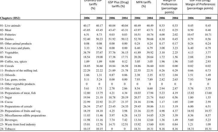
Table 7 compares the level of GSP tariffs and the margin of preferences for each group

of HS2-digit agricultural products for the years 2004 and 2006.9 The data allows us to observe

whether, and to what extent, tariffs differed across sectors, trade arrangements and from one year

to another. By limiting the discussion to the margin of preferences, it can be noticed that, as

expected, there are relevant differences between the ordinary GSP and the GSP-Drug.

Furthermore, the preferential margin is quite stable in 2004 and 2006 (the major changes

™occurred in fisheries [from 3.99% to 2.01% ], vegetables [3.1%; 2.25%], preparations of meat

[5.22%;4.19%]). The agricultural sectors with the highest margins of preference under the

ordinary GSP regime were tobacco (about 8.16% in 2006), preparations of meat (5.22% in

9

(17)

16 2006), preparations of fruits and vegetables (4.98% in 2006) and fisheries (3.99% in 2006). The

average margin was modest in the chapters of livestock, meat, dairy products, other animal

products, cereals, products of the milling industry, oilseeds, sugar, and residues and waste from

the food industry. To sum up, the level of the preferential tariff granted by the GSP did not

change much as a result of the introduction of the 2006 GSP scheme (on average, less than one

(18)

17

Level of the Duty Number of Tariff Lines %

Preferential Margin under Ordinary GSP

(Min‐Max)

Preferential Margin under GSP‐Drug

(Min‐Max)

Preferential Margin under EBA (Min‐

Max)

Total 3683 100 0 < marg < 175.22 0 < marg < 184.76 0 < marg < 184.76 >20% 973 26 0 < marg < 175.22 0.14 < marg < 184.76 8.86 < marg < 184.76 10‐20% 958 26 1 < marg < 16.97 1.3 < marg < 19.97 1.68 < marg < 19.97

5‐10% 603 16 0.5 < marg < 9.71 0.16 < marg < 9.94 3.84 < marg < 9.94 1‐5% 602 16 0.09 < marg < 4.36 0.6< marg < 4.96 1.15 < marg < 4.16 <1% 547 15 0 < marg < 0.97 0 < marg < 0.97 0 < marg < 0.97

Source: own computation based on data from DBTAR (2006) and Taric.

(19)

[image:19.842.59.787.50.491.2]

18

Table 7 Tariffs and Preferential Margins under GSP, by HS02-digit agricultural products (in %) (2004 and 2006).

Ordinary GSP tariffs

(%)

GSP Plus (Drug) tariffs (%)

MFN tariffs (%)

Ordinary GSP: Margin of Preferences (percentage

points)

GSP Plus (Drug) Margin of Preferences

(percentage points)

Chapters (HS2) 2006 2004 2006 2004 2006 2004 2006 2004 2006 2004

01- Live animals 40.17 40.17 40.04 40.04 40.49 40.49 0.33 0.33 0.45 0.45

02- Meat 43.85 43.45 43.47 43.31 43.97 43.71 0.12 0.25 0.50 0.40

03- Fisheries 6.51 8.73 0.03 0.03 10.51 10.74 4.00 2.02 10.47 10.71

04- Dairies 52.40 50.23 51.92 50.12 52.70 50.68 0.30 0.45 0.79 0.56

05- Other animal products 0.08 0.08 0.00 0.00 0.24 0.24 0.17 0.17 0.24 0.24

06- Live trees and plants 3.33 3.56 0.00 0.00 6.40 6.79 3.08 3.23 6.40 6.79

07- Vegetables 38.79 37.67 37.76 36.15 41.89 39.92 3.10 2.25 4.13 3.77

08- Fruits 18.54 19.08 17.38 17.71 20.26 20.64 1.72 1.56 2.88 2.94

09- Coffee, tea, spices 1.09 1.09 0.00 0.12 3.05 3.05 1.96 1.96 3.05 2.93

10- Cereals 18.85 36.60 18.84 36.58 18.86 36.60 0.01 0.00 0.02 0.02

11- Products of the milling ind. 22.29 22.22 21.89 21.78 22.55 22.51 0.26 0.29 0.66 0.73

12- Oilseeds 1.66 1.31 0.87 0.86 2.38 2.35 0.72 1.04 1.51 1.49

13- Lac, gums, resins 5.11 5.24 0.00 0.00 7.93 7.89 2.82 2.65 7.93 7.89

14- Other vegetable products 0 0 0 0 0 0 0 0 0 0

15- Oils and fats 5.61 5.73 2.78 2.86 8.54 8.60 2.94 2.87 5.76 5.75

16- Preparations of meat, fish 12.80 13.75 4.21 4.34 18.03 17.94 5.23 4.19 13.82 13.60

17- Sugar 19.94 21.18 18.78 20.19 20.57 21.74 0.63 0.56 1.80 1.55

18- Cocoa 22.99 22.92 21.27 21.37 24.16 23.96 1.17 1.05 2.89 2.59

19- Preparations of cereals 26.34 27.67 23.45 24.35 29.45 30.86 3.11 3.19 6.00 6.51

20- Preparations of fruits and veg. 18.19 18.18 4.25 3.98 23.16 22.55 4.98 4.37 18.92 18.57

21- Miscellaneous edible preparations 11.03 11.46 5.97 6.28 14.33 14.85 3.29 3.39 8.36 8.57

22- Beverages 11.98 11.16 7.74 7.42 13.34 12.64 1.36 1.49 5.60 5.23

23- Waste from food industry 15.01 12.76 14.71 12.51 15.92 13.60 0.91 0.84 1.21 1.09

24- Tobacco 10.15 10.15 0 0 18.31 18.31 8.16 8.16 18.31 18.31

(20)

19

VI. The gravity equation

The gravity model is widely used to explain the pattern of bilateral trade between nations and its

formulation is based on the idea that trade is positively influenced by the economic mass of the

trading countries and negatively affected by the geographical distance between them. Again,

trade flows are subject to trade resistance factors which can be improved by preferential trade

arrangements, such as the EU GSP.

The basic specification of the gravity equation used in the estimation is the following:

(1) ijl t ijl t ijl t ijl t ijl t ijl t ij ij ij ij j t i t j t i t ijl t u MED ACP EBA Drug GSP GSP Border Language Colony Dist POP POP GDP GDP M + + + + + − + + + + + + + + + + + + = ) ln( ) ln( ) ln( ) ln( ) ln( ) ln( ) ( ) ln( ) ( ) ln( ) ln( 13 12 11 10 9 8 7 6 5 4 3 2 1 β β β β β β β β β β β β β α

where subscript i refers to the importing countries, which, in our case, are the members of

EU-15; j refers to the exporting country; l to the product line; t is time. The notation is defined as

follows: M_ijlt are the exports of products l from country j to country i at time t; GDP_it and

t j

GDP represent the economic size of country i and country j at time t;POP_it and POP_jt are the

populations of the two countries at time t; DIST_ij is the distance between the locations measured

from capital to capital; Language is a dummy that takes value 1 if countries i and j speak the

same language, and 0 otherwise; Colony is a dummy that takes value 1 if colonial links exist (or

have existed) between countries i and j, and 0 otherwise; Border is a binary variable assuming

the value 1 if countries i and j share a common land border, and 0 otherwise; uijlis a composite

error term.

As mentioned above (cfr § 1), for the purpose of this study, we have to address the

crucial issue of the measure of the trade preferences, which, in the related literature, have been

often captured through dummy variables, which are equal to one if the exporting country belongs

to a PTA and zero otherwise. Thus, their coefficient is expected to be positive because preferred

countries should export more than non-preferred countries. However, this approach is not wholly

satisfactory because dummies treat all preferences as a homogeneous group, without taking into

account their specific characteristics. Furthermore dummies do not distinguish between different

preferential instruments, such us preferential margins, quotas and entry prices. Finally, they do

(21)

20 There have recently been some studies that have used preferential margin or tariffs to

assess potential benefits deriving from preferential schemes (Cardamone, 2009; Cipollina and

Salvatici, 2007; Emlinger et al., 2009). Some of these studies (Cardamone, 2009; Cipollina and

Salvatici, 2007) have calculated the preferential margin as the difference between the highest

tariff applied by the EU and the duty paid by an exporter for a given product. While Cipollina

and Salvatici (2007) do not distinguish between different preferential margins, Cardamone

(2009) does. Emlinger et al., 2009 used the tariffs rather than the preferential margin to measure

the preferences granted. Following these recent papers and in order to overcome many of the

shortcomings related to the dummy approach, this paper employs a quantitative measure of the

trade preferences and, in this sense, the other elements in eq. [1] (GSP, GSP-Drug, EBA, ACP,

MED) become the key variables of our analysis. They represent the preferential margin

established under a given agreement in favor of a country when exporting certain commodities to

the country giving preferences. For instance, GSP_ijlt is the preferential margin under the ordinary

GSP that the j-th country enjoys at time t when exporting product line l to country i. The same

applies for the other preference variables (GSP-Drug, EBA, ACP and MED). For each trade

agreement, the preferential margin is defined as the ratio between the preferential margin (the

difference between the MFN and the preferential duties at each tariff line) and the MFN tariff.

The formula is:

l ijt

l ijt l

ijt l

ijt

MFN

F

PREF_TARIF

MFN

alMargin

Preferenti

=

−

(2)

where i refers to importers, who, in our case, are the members of EU-15, j indicates the exporting

countries, l is the tariff line and t is time. PREF_TARIFF indicates the preferential tariffs applied

under the specific trade arrangement (GSP, GSP-Drug, EBA, ACP, MED). This measure allows

us to take into account the size of the actual tariff preference for a particular product.10 The

overlapping of preferences has been solved by taking for a given trade flow the maximum

margin of preference as that which has been used by the beneficiary country. For instance, if a

country is eligible for preferential treatment under both the GSP and the Cotonou agreement, and

10

(22)

21 the preferential margins are, respectively, 3% and 5%, we assume that country will export under

the Cotonou agreement and set the GSP preferences equal zero.

The econometric analysis considers the imports of each EU-15 member of HS6-digit 763

agricultural products (cfr footnote 3) from 169 exporters (the exporting countries are listed in

Appendix A). In estimating the eq. [1] we consider the 4-year period 2001-2004, and this time

coverage is due to the availability of data on tariffs for the very large set of products. The only

dataset which makes a large amount of statistics easily available on tariffs, such as the ones we

need to run our regressions at HS6-digit level, is DBTAR (2006) and this source covers the

period 2001-2004.

VII. Econometric issues and the estimation method

In estimating a gravity model, there are three econometric issues to be addressed which are

related to the non-observable heterogeneity of countries and to sample selection bias.

With regards country heterogeneity, it ought to be said that it introduces bias into the

estimation because of the likely correlation between non–observable, country-specific effects

and the explanatory variables of the gravity equation. Heterogeneity may be due to observable

and unobservable factors (such as the propensity of one country to export more than others,

cultural and historical links or business cycle effects), and/or to several other aspects which

define each country-pair background (i.e., common language, colonial past, shared border or

religion). While this background based on observable factors can be handled by using a set of

dummy variables, it is necessary to use a model with country fixed effects to control for

non-observable factors (Serlenga and Shin 2007). In order to take into account countries’

heterogeneity, we have decomposed the error term of equation (1) as follows:

(3)

where αi and αj refer to time-invariant importer and exporter-country fixed effects,

respectively, α_l to commodity fixed effects, α_t to time fixed effects and finally εtijl is an

idiosyncratic error term. The fixed effects were meant to capture all unobserved factors that

influence export flows, while the time variable allowed us to control for macro-economic factors

that may have occurred over our sample period.

As far as sample selection bias is concerned, it must be pointed out that there is a long

tradition of using a log-linearization of gravity equations. However this procedure fails when

zero trade observations are present and will lead to biased estimates. There is a great deal of

evidence that zeros are frequent in bilateral trade. For instance, Haveman and Hummels (2004)

ijl t t l j i ijl t

(23)

22 find that almost 1/3 of bilateral trade flowing between 173 countries in 1990 was zero, while

Helpman et al. (2008) show that about half the country pairs in their sample of 158 trading

countries did not trade with each other from 1970 to 1997. In our case, because of the product

disaggregation, zeros extend to 90% of the entire sample. Therefore, dropping zeros implies a

loss of useful information as to why some countries trade in certain sectors and not in others.

The issue of zero-trade flows has been widely addressed in the literature on gravity

empirics (Martinez-Zarzoso et al., 2007; Martin and Pham, 2008; Santos Silva and Tenreyro,

2006). In particular, Santos Silva and Tenreyro (2006) contribute to the discussion as to which

estimator provides the most reliable results by assessing the potential bias of elasticities in a log

linearised regression. They show that the consistency of an OLS estimator depends on a

restrictive assumption regarding the error terms and suggest that the gravity equation could be

estimated in its multiplicative form by using the Pseudo Quasi Maximum Likelihood Method

(PQML) based on a Poisson Model. Moreover since the standard Poisson model is vulnerable to

problems such as over-dispersion and excess zero flows, we have used other estimation

techniques, i.e. the Zero Inflated Poisson (ZIP) and the Negative Binomial Regression (NBR), as

in Burger, van Oort, and Linders (2009).

More precisely, Santos Silva and Tenreyro (2006) argue that linearisation of the gravity

equation in the presence of heteroskedasticity leads to inconsistent estimates because the

expected value of the logarithm of a random variable depends both on its mean and on

higher-order moments of its distribution. Hence, if variance of the error term depends on regressors, the

expected value of the error term logarithm will also depend on the regressors, violating the

condition of consistency of OLS. The PML allows us to estimate the gravity equation and, more

generally, constant elasticity models in their multiplicative form, and to allow for

heteroskedasticity. However, an important condition of the Poisson model is equi-dispersion. In

many cases, though, the conditional variance is normally higher than the conditional mean,

which implies that the dependent variable is over-dispersed. The Poisson regression model only

accounts for observed heterogeneity, where different values of the predictor variables result in a

different conditional mean value. Unobserved heterogeneity, however, originates from omitted

variables; if we do not take into account unobserved heterogeneity, the results are inconsistent

and inefficient. In order to correct for over-dispersion, a negative binomial regression model can

be used. The expected value of the observed trade flow in the negative binomial regression

model is the same as in the Poisson regression model, but the variance here is specified as a

function of both the conditional mean and a dispersion parameter. In other words, an additional

error term has been added to the negative binomial regression model. The standard errors in the

(24)

23 small p-values (Cameron and Trivedi, 1986, 31). The Zero-Inflated model accounts for two

latent groups within the population: a group with zero counts and a group with a non-zero

probability of having counts other than zero. As Burger et al. (2009, p. 175) summarise: these

models “take into account that not all pairs of countries have the potential (or are at risk) to trade

because of trade embargos or a severe mismatch between demand and supply. On a similar note,

the geographical or cultural distance between countries may simply be too large for trade to be

profitable. Hence, the profitability of trade, which reflects the trade potential, can be separated

from the volume of trade as stemming from two different processes”.

To sum up, we have evaluated the preferences for agro-food products (from HS01 to

HS24) granted by the EU under its GSP scheme from 2001 to 2004 using five different

estimators (OLS, LSDV, PQML; ZIP and NBR), the results of which are presented in the

successive section.

VIII. Results

In this section, we have summarised the results obtained when estimating equation [1] with the:

the OLS, LSDV, PQML, NBR (Negative Binomial Regression) and the ZIP (Zero Inflated

Poisson) procedures. The first estimations we made regarded the pooled data of all agricultural

exports to the EU. Afterwards we ran separate regressions for the following groups of products:

livestock, fisheries, fruits, lacs and gums, oils and fats, products of animal origin, sugar,

vegetables, beverages and spirits, tobacco, tropical fruits and residues from the food industry.

Whatever the estimation, the trade statistics used are identified at HS6- digit level. The results

for the pooled data are presented in table 8, while those obtained sector-by-sector are presented

in table 9.

The first five columns of table 8 show the results obtained when equation [1] is estimated

using the aforementioned methods. By comparing the outcomes, it emerges that the estimated

parameters differed both in sign and magnitude. Briefly, when focussing on gravity standard

variables, we found that the elasticity of importing country GDP was always positive and

statistically significant in OLS (column 1), Poisson (column 3) and NBR (column 4) estimates.

On the other hand, exporting country GDP was only found to exert a significant (and negative)

impact in OLS results. As for the observable country-pair variables, we found that the best

performing estimators were the Poisson and the NBR. It was only then, indeed, that some

variables (Distance, Colonial Ties and Common Language) showed the expected signs and were

(25)

24 regressions. This was the case with Border, for instance, where, when significant, a negative sign

emerged.

With regards to the goal of this work, we found that the GSP preferential scheme exerted

a positive and significant impact on beneficiary countries in all the regressions and was

significant in OLS, LSDV and ZIP regressions. When significant, its estimated value ranged

from 0,024 (ZIP regression) to 0,061 (LSDV estimates), whereas the estimate was 0.042 with the

OLS. The same applied for the EBA initiative, whose coefficient was 0.025 in OLS results,

0.038 in the ZIP regression and 0.086 when considering the LSDV estimator. The estimated

coefficient of the GSP-Drug was significantly positive only when using the LSDV, while it

turned out to be negative in the OLS and the ZIP regression (although in this case the

significance was at the 10% level). Little encouraging evidence was found for the impact of the

EuroMed agreement, which, at best, was positive and significant only in the LSDV regression.

Finally, the preferential margin granted under the Cotonou Agreement in favour of ACPs

positively affected the agricultural exports of beneficiaries only when the gravity model was

estimated using the OLS and the LSDV techniques (table 8).

Overall, the evidence emerging is mixed. On the one hand, the only clear indication

comes in the form of the positive impact exerted by the Ordinary GSP. On the other hand, the

only results regarding the impact of all of these preferential agreements are those obtained from

the LSDV method. As can be seen in table 8, this estimator yields statistical and positive

coefficients whatever the trade preference and, in this sense, one conclusion that can be drawn is

that the largest impact was the one brought about by the EBA initiative (the estimated parameter

is 0.086), followed by the ordinary GSP (0.061), Med (0.02), GSP-Drug (0.012) and, finally, by

the Cotonou agreement (0.009).

In order to check the robustness of results, we have re-estimated our models by replacing

the five separate variables measuring the preferential margins (Ordinary GSP, GSP-Drug, EBA,

ACP and EuroMed) with the variable named MaxPref, which corresponds to the maximum

margin of preference observed for each export flow. The rationale behind this variable is to

address the overlapping of preferences by assuming that any trade flow is determined by only

one trade agreement, i.e. by the one assuring the largest preference margin. This is similar to

what we did before when addressing the issue of preference overlapping (cfr § VI), but in this

case we use a single, common vector, MaxPref, instead of five different preferential variables.

The use of this variable is meant to provide an overall assessment of the effectiveness of the

trade preferences granted by the EU. The estimation outcomes, which are summarised in table 8,

indicate that the sign of the coefficient of MaxPref is always positive, although is only

(26)

25 tends to support the view that EU trade preferences help DCs export more to European

agricultural markets.

Finally, in the following we limit the presentation of the results obtained when running

the gravity regression for each agricultural sector to those related to the Zero Inflated Poisson

Regression. The estimates are displayed in table 9.

In comparing results between agricultural groups, we found that the GDP coefficient for

importing countries is positive and statistically significant in two cases, oils-fats and residues

from the food industry, while it is negative and not significant in the other group of products.

The GDP coefficient for exporting countries is negative and significant in all regressions except

for tobacco, where it is positive and significant. The population coefficient of importing

countries has an ambiguous sign, as well the population coefficient of exporting countries.

Distance is unexpectedly positive and significant in the case of live trees, fruits, oils-fats and

tropical fruits, at a level of significance of 1%. Border, colony and language have ambiguous

signs.

With respect to the preferential margin, the coefficient for the GSP presents a positive

coefficient for the following agricultural groupings: live Trees (0.036), sugar (0.020), fruits

(0.019), tropical fruits (0.038) and residues from the food industry (0.036), and a negative and

significant coefficient for beverages-spirits (-0.084) and oils-fats (-0.204). The GSP-Drug shows

positive and significant coefficient in oils-fats (0.054) and beverages-spirits (0.018), while it

reports a negative and significant coefficient for residues from the food industry (-0.064) and

live trees (-0.012). The EBA special initiative only has a positive and significant coefficient for

lacs-gums (0.049), while, in the other groupings, its coefficient is positive but not statistically

significant. The ACP coefficient is positive and significant for the following products: fruits

(0.027), vegetables (0.012), lacs-gums (0.036) and beverages-spirits (0.031). The Mediterranean

preferential margin is positive and significant for tropical fruits (0.028) and beverages-spirits

(0.023), while it is negative and statistically significant for tobacco (-0.034). Nothing can be said

with regards other products (fisheries and products of animal origin) since the Zero Inflated

Poisson Regression does not converge.

Based on these results, it may be argued that the evidence revealed regarding the sector

by sector impact of trade preferences is puzzling. The impact of the GSP scheme is effective in

increasing DC exports to EU of live trees, sugar, fruits, tropical fruits and residues from the food

industry, while the GSP-Drug and the EBA are able to increase DC exports of oils and fats,

beverages-spirits and lacs-gums. The Cotonou agreement is effective in increasing the exports of

fruits, vegetables, lacs-gums and beverages-spirits, while the EuroMed agreement is effective in

(27)

26

Table

8 UE

‐

15 Agricultural

Imports

and

the

impact

of

the

EU

GSP

scheme.

Estimates

of

a

gravity

equation

when

using

the

OLS,

LSDV,

Poisson,

NBR

and

the

ZIP

methods

(2001

‐

2004).

OLS LSDV POISSON NBR ZIP OLS LSDV ZIP

GDP IMPORTER 0.841*** 0.119 1.469*** 2.900*** 0.180 0.889*** 0.142 1.491***

[0.016] [0.257] [0.291] [0.636] [0.415] [0.017] [0.256] [0.291]

GDP EXPORTER -0.102*** -0.013 0.010 0.004 -0.008 -0.027*** 0.043 0.033*

[0.004] [0.038] [0.020] [0.051] [0.044] [0.003] [0.037] [0.018]

POP IMPORTER -0.065*** -0.644 -2.921** 2.944 -0.163 -0.114*** -0.824 -2.874**

[0.016] [1.058] [1.372] [3.938] [1.564] [0.017] [1.055] [1.362]

POP EXPORTER -0.091*** 0.530 -0.564 -1.561** -0.247 -0.148*** 1.087** -0.262

[0.004] [0.436] [0.659] [0.739] [0.550] [0.004] [0.431] [0.655]

DISTANCE 0.079*** 0.230*** -0.400*** -0.636*** 0.277*** 0.083*** 0.227*** -0.401***

[0.006] [0.017] [0.068] [0.091] [0.027] [0.005] [0.017] [0.068] GSP 0.042*** 0.061*** 0.021 0.002 0.024***

[0.002] [0.003] [0.023] [0.023] [0.003]

GSP DRUG -0.016*** 0.012*** -0.015 -0.045 -0.007*

[0.002] [0.004] [0.019] [0.028] [0.004]

EBA 0.025*** 0.086*** 0.042 0.010 0.038***

[0.002] [0.003] [0.035] [0.040] [0.004]

ACP 0.010*** 0.009*** -0.021 -0.038* -0.022***

[0.002] [0.002] [0.018] [0.023] [0.002]

MED -0.021*** 0.020*** -0.012 -0.028* -0.008*

[0.002] [0.004] [0.013] [0.017] [0.005]

BORDER -0.274*** -0.014 -0.375*** 0.032 0.022 -0.206*** -0.016 -0.375***

[0.023] [0.028] [0.070] [0.095] [0.040] [0.022] [0.028] [0.070]

LANGUAGE -0.157*** -0.181*** 0.265*** 0.276*** -0.154*** -0.086*** -0.184*** 0.265***

[0.017] [0.019] [0.058] [0.105] [0.025] [0.016] [0.019] [0.058]

COLONY -0.002 -0.015 0.365*** 0.699*** -0.025 -0.022 -0.019 0.365***

[0.016] [0.018] [0.034] [0.066] [0.023] [0.015] [0.018] [0.034]

MAXPREF 0.037*** 0.054*** 0.010

[0.001] [0.001] [0.018]

CONSTANT -6.431*** 8.162 32.089 -76.210 11.869 -7.959*** -1.550 18.813

[0.200] [14.864] [21.423] [72.470] [20.250] [0.199] [14.793] [18.904]

OBSERVATIONS 175884 175884 3712014 3712014 3712014 175884 175884 3712014

R-squared 0.193 0.245 0.197 0.249