Asset Price Bubbles in the Kiyotaki Moore Model

Munich Personal RePEc Archive

Asset Price Bubbles in the

Kiyotaki-Moore Model

Hirano, Tomohiro and Inaba, Masaru

December 2010

Asset Price Bubbles in the Kiyotaki-Moore

Model

∗

Tomohiro Hirano

and Masaru Inaba

First Version, December 2010

This Version, December 2011

Work in Progress

Abstract

We examine the effect of asset price bubbles in the Kiyotaki-Moore model. We show that the dynamic interactions between bubble-asset price, land price, and output generate powerful bubbly dynamics. The boom-bust cycles in bubble-asset price cause boom-crash cycles in the land market simultaneously, like a contagion by affecting the funda-mentals of land. We also numerically analyze the welfare effects of bubbles in transitional dynamics.

Key words: Bubbly Dynamics, Contagion, Welfare Effects of Bub-bles

∗_{We have benefited greatly from discussions with Toni Braun and Masaya Sakuragawa.} †_{Faculty of Economics, The University of Tokyo, tomohih@gmail.com}

‡_{Faculty of Economics, Kansai University, and The Canon Institute for Global Studies,}

1

Introduction

Many countries have experienced bubble-like dynamics. The boom-bust in asset prices in equity markets tends to be associated with the boom-crash of land or housing markets, which, in turn, has large effects on real economic activity. Notable examples include the U.S. before and after the financial crisis of 2007–2008 and Japan from the late 1980s to the beginning of the 1990s.1

The episodes in these countries suggest that financial markets are connected to each other, in the sense that the boom and collapse in one asset market has contagious effects on other asset markets.

In this paper, we theoretically investigate contagious effects of asset price bubbles on the other asset market. For this purpose, we incorporate a bubble-asset into the model of Kiyotaki and Moore (1997). Following traditional literature such as Tirole (1985), this asset produces no real dividend, i.e., the fundamental value of the asset is zero. One interpretation of the asset is that an equity with no dividends circulates. We first show that the dynamic inter-actions between bubble-asset price, land price, and output generate powerful bubbly dynamics. Second, the boom-bust cycles in bubble-asset price cause boom-crash cycles in the land market simultaneously, like a contagion, by affecting the fundamentals of land.

Figure 1 shows the mechanisms of the dynamic interactions in a bubbly episode. Output, land price, and bubble-asset price interact with each other not only within a period, but also between periods. This dynamic interaction between asset prices and aggregate quantity is similar to the Kiyotaki-Moore model. The key innovation of our paper is that the presence of bubbles enhances this interaction, increasing investment, output, consumption, and land price compared to the bubbleless economy. Once a bubble collapses, a reversal mechanism operates. Investment, output, consumption, and land price all fall eventually.

[Insert Figure 1]

A feature of bubbly equilibrium is that bubbles affect the land market by changing fundamentals of land itself, i.e., cash flows from land. In the bubbleless economy, land allocation is inefficient, in the sense that even un-productive entrepreneurs use land to produce goods as in Kiyotaki and Moore

1

(1997). As a result, output, investment, consumption, TFP, and land price are all low in the steady-state bubbleless economy. Bubbles not only in-crease the net worth of entrepreneurs facing the borrowing constraint, but also improve land allocation, i.e., more land is used in productive sectors. This improves cash flows from land and increases land price, which in turn relaxes credit limits, thereby generating expansionary effects.

Although bubbles improve resource allocation and produce expansionary effects, are they welfare-improving or welfare-reducing? We also investigate welfare effects of bubbles. Traditional wisdom such as Tirole (1985) suggests that bubbles are welfare-improving. In his framework, although bubbles increase consumption, they are contractionary in investment and output. On the other hand, Grossman and Yanagawa (1993) shows that bubbles are welfare-reducing. In their model, consumption, investment, and output all decrease by bubbles. This contractionary view has been criticized, because it seems to be inconsistent during bubbly episodes. We investigate welfare effects within a framework in which bubbles are expansionary in all three variables. Kocherlakota (2009) also examines welfare effects of bubble in the expansionary case. The difference between his analysis and ours is that we consider welfare effects including transitional dynamics, while he focuses on welfare in the steady state.

Our paper is related to a number of recent theoretical studies on rational asset price bubbles. Since a seminal paper by Farhi and Tirole (2009), the recent literature have provided a theoretical framework to analyze expansion-ary effects of asset price bubbles. Examples include Hirano and Yanagawa (2010a, 2010b), Martin and Ventura (2010, 2011), Aoki and Nikolov (2011), Ventura (2011), Miao and Wang (2012), and Sakuragawa (2012).2

These studies only have one asset market, bubble-asset market.3

Different from these studies, our model has two asset markets, bubble-asset market and land market. Thus, we can analyze interactions between two asset markets, and investigate contagious effect of changes in the bubble-asset market on the land market.

Kocherlakota (2009) and Miller and Stiglitz (2010) are closely related to our study, in the sense that they examine the effects of boom-bust cycles of bubbles in the Kiyotaki-Moore model. There are significant differences. In

2

Kocherlakota (1992), Santos and Woodford (1997), and Hellwig and Lorenzoni (2009) analyze asset price bubbles in an endowment economy with an infinitely lived agent.

3

Kocherlakota’s model, land is not used as a factor of production and does not produce any output, i.e., the fundamental value of land is zero. He analyzes the case of positive land price as a bubbly economy. On the other hand, in our model, land is used as a factor of production. Miller and Stiglitz describe bubbles as corrective error of forecast on land price. In contrast, our model is based on a rational bubble model.

The paper is organized as follows. In section 2, we present a basic model and then derive the existence condition of bubbles. We also compare the bubble economy to the bubbleless economy in the steady state. In section 3, we analyze bubbly dynamics and discuss the welfare implications of bubble.

2

The Model

We develop an infinitely lived agent model in which the financial market is imperfect. Our model is based on Kiyotaki and Moore (1997).

2.1

Entrepreneur’s Problem

Consider a discrete-time economy with a continuum of entrepreneurs. A typical entrepreneur has the following expected discounted utility:

E0

[ ∞

∑

t=0

βt

logci t

]

, (1)

where i is the index for each entrepreneur and ci

t is his or her consumption

in period t. β ∈ (0,1) is the subjective discount factor and E0[·] is the

conditional expectation on information at the beginning of period 0.

In each period, each entrepreneur has high production opportunities to produce the homogeneous goods (hereinafter H-projects) with probability

p, and low production ones (L-projects) with probability 1 − p.4

Both high- and low-productivity entrepreneurs (hereafter, H-entrepreneurs and L-entrepreneurs) use land and intermediate goods as inputs to produce the homogeneous goods. The land has a fixed supply, which is normalized to be one. The intermediate goods fully depreciate one period after production.

4

The production technologies are as follows:

yit+1 =α

i t ( ki t σ

)σ(

zi t

1−σ

)1−σ

, (2)

where ki

t(≥ 0) is land, z i

t(≥ 0) is intermediate goods in period t, and y i t+1

is output in period t+ 1. αi

t is productivity in period t. α i t = α

H

if the entrepreneur has H-projects, and αi

t = α L

if he or she has L-projects. We assume αH

> αL

. The probability p is exogenous and independent across entrepreneurs and over time. At the beginning of each period t, the en-trepreneur knows his or her own type in period t, whether he or she has H-projects or L-projects. Assuming that the initial population measures of H-types and L-types are p and 1−p, respectively, the population measures in subsequent periods are the same.

In this economy, we introduce bubbles. We define a bubble-asset as an asset that produces no real return, i.e., the fundamental value of the asset is zero. Let Pt be the per unit price of bubble-asset in period t in terms

of consumption goods. Then, the entrepreneur’s flow of funds constraint is given by

ci

t+qt(k i t−k

i

t−1) +z

i

t+Pt(x i t−x

i

t−1) +rt−1b

i

t−1+qtγk i t−1 =y

i t+b

i t, (3)

where xi

t is the amount of bubble-asset purchased in period t. The left

hand side of (3) shows expenditure on consumption, net purchase of land, investment of intermediate goods, net purchase of bubble-asset, repayment, and maintenance costs. As in Lorenzoni (2008), we assume that in order to keep the land productive, each entrepreneur must pay maintenance costs for a proportion γ of his or her land holdings. The right-hand side shows the available funds in period t, which includes the return from investment in the previous period and new borrowing. We define the net worth of the entrepreneur in period t asei

t ≡y i

t−rt−1b

i

t−1+qtk i

t−1(1−γ) +Ptx i t−1.

We assume that because of frictions in the financial market, the en-trepreneurs are credit-constrained. Following Kiyotaki and Moore (1997), creditors limit credit so that debt repayment cannot exceed the value of col-lateral, i.e., the value of the land minus maintenance costs. That is, the borrowing constraint becomes

rtb i

t≤qt+1k

i

t−qt+1γk

i

whereqt+1 is the price of land in periodt+ 1. rt and b i

t are the gross interest

rate and the amount of borrowing in period t, respectively. We also impose a short sale constraint on bubble-asset:5

xi

t ≥0. (5)

2.2

Equilibrium

Let us denote the aggregate consumption of H- and L-entrepreneurs in period

t as ∑

i∈Htc

i t ≡ C

H t and

∑

i∈Ltc

i t ≡ C

L

t , respectively, where Ht and Lt are

families of H- and L-entrepreneurs in periodt. Similarly, let∑

i∈Htz

i t ≡Z

H t ,

∑

i∈Ltz

i t ≡Z

L t ,

∑

i∈Htb

i t ≡ B

H t ,

∑

i∈Ltb

i t ≡B

L t ,

∑

i∈Htk

i t ≡K

H t ,

∑

i∈Ltk

i t ≡

KL t ,

∑

i∈Ht∪Ltx

i

t≡Xt,and

∑

i∈Ht∪Lty

i

t ≡Ytbe aggregate investment,

aggre-gate borrowing, aggreaggre-gate land holdings, and aggreaggre-gate demand for bubble-asset of each type, respectively. Assuming that the aggregate supply of bubble-asset is fixed over time X, then the market clearing conditions for goods, credit, land, and bubble-asset are, respectively,

CH t +C

L t +Z

H t +Z

L

t =Yt−qtγ, (6)

BH t +B

L

t = 0, (7)

KtH +K L

t = 1, (8)

Xt=X. (9)

The competitive equilibrium is defined as a set of prices{rt, qt, Pt} ∞ t=0 and

quantities{

ci t, b

i t, z

i t, x

i t, k

i t, C

H t , C

L t , B

H t , B

L t , Z

H t , Z

L t , K

H t , K

L t, Yt

}∞

t=0, such that

(i) the market clearing conditions, (6)-(9) are satisfied, and (ii) each en-trepreneur chooses consumption, borrowing, land holdings, investment of intermediate goods, and bubble-asset to maximize his or her expected dis-counted utility (1) under the constraints (2), (3), (4), and (5). Because there is no aggregate uncertainty, the entrepreneurs have perfect foresight of future prices and aggregate quantities in equilibrium. We also rule out the explosion in land price:

lim

t→∞

qt(1−γ) t

r0r1r2· · ·rt−1

= 0. (10)

5

As is well known, there are multiple equilibria in the rational bubble model. One is the equilibria with Pt >0; the other isPt = 0. In the rest of

the analysis, we focus on Pt > 0 and analyze what happens in the bubble

economy.

2.3

Entrepreneur’s Behavior

We are now in a position to characterize the equilibrium behavior of en-trepreneurs in the bubble economy. We consider the case

αL

uσ t

< rt<

αH

uσ t

, (11)

whereut≡qt−qt+1(1−γ)/rt is the opportunity cost, or user cost, of holding

land from t to t+ 1. αL

/uσ

t and α H

/uσ

t are the rates of return of L-projects

and H-projects, respectively.

In order that bubble-asset be held in equilibrium, the rate of return of bubble-asset must be equal to the interest rate:

rt =

Pt+1

Pt

. (12)

When (11) and (12) hold, both the borrowing constraint and the short sale constraint simultaneously become binding for entrepreneurs who have H-projects in period t, but not for entrepreneurs who have L-projects. Since the utility function is logarithmic, each entrepreneur consumes a fraction 1−β of the net worth in each period, that is,

ci

t = (1−β)

[

yi

t−rt−1b

i

t−1+qtk i

t−1(1−γ) +Ptx i t−1

]

. (13)

Then, by using (3), (4), and (5), we can derive demand functions of the type i agent of H-entrepreneurs for intermediate goods and land holdings in period t:

zi

t = (1−σ)β

[

yi

t−rt−1b

i

t−1+qtk i

t−1(1−γ) +Ptx i t−1 ] , (14) ki t = σβ[ yi

t−rt−1b

i

t−1+qtk i

t−1(1−γ) +Ptx i t−1

]

qt−

qt+1(1−γ)

rt

Equation (14) indicates that H-entrepreneur spends a fraction 1−σ of his or her savings on intermediate goods. Equation (15) indicates that H-entrepreneur spends a fraction σ of his or her savings to finance the dif-ference between the land value qt and the collateral value qt+1(1−γ)/rt.6

The difference qt−qt+1(1−γ)/rt is the down payment to purchase one unit

of land, and is the user cost ut. The entrepreneurs buy bubble-asset when

they have L-projects, and sell them when they have opportunities to invest in H-projects. As a result, their net worth increases (compared to bubbleless cases), which boosts their demand for intermediate goods and land as shown in (14) and (15).

L-entrepreneurs in period t prefer buying bubble-asset and lending to H-entrepreneurs instead of investing in their own L-projects when (11) and (12) hold because the rate of return of bubble-asset or lending is greater than the rate of return of L-projects.

2.4

Aggregation

Since (14) and (15) are linear functions of net worth, we can the aggregate across H-entrepreneurs to derive the aggregate demand functions:

ZH

t = (1−σ)βp[Yt+qt(1−γ) +PtX], (16)

KH t =

σβp

qt−

qt+1(1−γ)

rt

[Yt+qt(1−γ) +PtX], (17)

where Yt +qt(1− γ) +PtX is the aggregate wealth of the entrepreneurs.

Since every entrepreneur has the same chance to take on H-projects in each period, a proportion pof aggregate wealth is the wealth of H-entrepreneurs. Equation (16) and (17) indicate that the aggregate demand functions for intermediate goods and land depend upon cash flow from investments in the previous period Yt as in Bernanke and Gertler (1989) and land price qt as

in Kiyotaki and Moore (1997). What is new in our framework is that the demand functions also depend upon bubble-asset price Pt, i.e., the presence

6

of bubbles increases demands for land holdings and intermediate goods, does not crowds them out as in traditional literature (Tirole (1985)).

Since only H-entrepreneurs use land, from the land market clearing con-dition,

σβp[Yt+qt(1−γ) +PtX]

qt−

qt+1(1−γ)

rt

= 1. (18)

Note that qt is an increasing function ofPt, Yt,and qt+1. When Pt increases,

the net worth of H-entrepreneurs improves. As a result, they can buy more land with maximum leverage, which raises the current land price qt.

More-over, when qt+1 is expected to increase, the borrowing constraint is relaxed,

which increases the demand for land, as in the model of Kiyotaki and Moore (1997). In our model, qt+1 is affected by the bubble-asset price in period

t+ 1, Pt+1.

From the aggregate flow of funds constraint of L-entrepreneurs and the market clearing condition for bubble-asset (9), we can derive the equilibrium the bubble-asset price in period t:

PtX=

β(1−p) [Yt+qt(1−γ)]−B H t

1−β+pβ (19)

We see that given BH

t , Pt is an increasing function of Yt and qt. Intuitively,

when cash flow or land price increases, the net worth of L-entrepreneurs improves and they can buy more bubble-asset, which raises the bubble-asset price.

Note that from (18) and (19), bubble-asset price Pt and land price qt

reinforce each other within a period. Moreover, as we will see, since both asset prices are forward-looking variables, they interact with each other between periods.

Since only H-entrepreneurs produce by using land and intermediate goods, output evolves over time as

Yt+1=

αH

σ u

1−σ

t . (20)

From the definition of the user cost of land and equation (12), the land price should satisfy the dynamic equation

qt=ut+

Pt

Pt+1

From this, the current land price equals the discounted value of future user costs, which in turn depends on the discounted value of future output from (20). This means that when output is expected to increase in the future, the current land price rises. Additionally, future output is affected by the presence of bubbles.

Since both H- and L-entrepreneurs consume a fraction 1−β of the net worth, goods market clearing condition (6) can be written as

(1−β)At+

1−σ

σ ut=Yt−qtγ, (22)

where At ≡ Yt+qt(1−γ) +PtX is aggregate wealth. The first term on the

left hand side of (22) is aggregate consumption and the second is investment of intermediate goods.

Along the perfect foresight equilibrium path, aggregate wealth evolves over time as

At+1 =

αH

uσ t

pβAt+

Pt+1

Pt

(1−p)βAt. (23)

Equation (23) indicates that given the aggregate savings of the economyβAt,

the aggregate net worth of H-entrepreneurs earns a rate of return αH

/uσ t,

while the net worth of L-entrepreneurs earns Pt+1/Pt.

2.5

Steady State Analysis

In order for bubbles to exist in the steady state, the following two conditions must be satisfied:

αL

uσ ≤1, (24)

P > 0. (25)

bubbleless economy, which means K′L t > 0.

7

From these conditions, we obtain the following proposition.

Proposition 1 Bubbles can exist if and only if the following condition is satisfied:

αH

≥ α

L

pβ

1−β+pβ, (26)

Proof. The proof is provided in the appendix A.

In order for bubbles to exist in the steady-state equilibrium, productivity

αH

must be sufficiently high. Intuitively, if productivity is high enough, the marginal productivity of production becomes lower, which means that the user cost becomes sufficiently large that the rate of return of bubble-asset becomes greater than the rate of return of L-projects.

We should add a few more remarks on maintenance costs. As in tradi-tional ratradi-tional bubble literature such as Tirole (1985) and Farhi and Tirole (2011), in the steady-state bubble economy with no growth, the interest rate equals one, in which case (10) cannot be satisfied in our model because our model has a fixed asset, land. In order that (10) is satisfied, we must intro-duce costs associated with land holdings.

Proposition 2 Output, investment, consumption, and aggregate TFP are all higher in the bubbly steady state than in the bubbleless steady state.

Proof. The proof is provided in the appendix B.

In the steady state of the bubbleless economy,8

production is inefficient in the sense that L-entrepreneurs as well as H-entrepreneurs produce by using land and intermediate goods, which means that resource allocation is ineffi-cient. On the other hand, in the bubbly steady state, only H-entrepreneurs produce. This means that a bubble increases efficiency in production by elim-inating inefficient L-projects, thus improving aggregate TFP. In other words,

7

The condition that L-entrepreneurs produce in the bubbleless economy is the following:

1−p(1−σ)−σp α

L

αL

−(1−γ) [αH

p+αL

(1−p)]β >0.

If this condition is satisfied, Pt>0 holds true.

8

the presence of bubbles helps transfer resources from L-entrepreneurs to H-entrepreneurs. Since resource allocation is more efficient, all macroeconomic variables are higher than those in the bubbleless steady state.

With regard to the effects of a bubble on land price, since only H-entrepreneurs produce in the bubbly steady state, cash flow from land in-creases from the present to the future, which raises the steady-state land price. On the other hand, the interest rate is high in the bubbly steady state, which decreases land price.9

In this sense, there are two competing effects of a bubble on land price. Which of these effects dominates depends on the value of γ.10

In the following example, we focus on the case where a bubble increases land price in the steady state.

An interesting feature in our framework is that bubbles changes funda-mentals itself, i.e., cash flow from land and interest rate. When the land price is higher in the bubble economy, it reflects an improvement in cash flow, and this improvement is supported by the presence of bubbles. This implies that boom-bust in bubble-asset price is associated with dramatic changes in fundamentals of land.

3

Macroeconomic Effects of Asset Bubbles

Given an initial condition Y0, the perfect foresight equilibrium path is

de-scribed by sequences {qt, At, rt, ut, Pt, Yt} ∞

t=0, satisfying (10), (20), (21), (22),

and (23). With regard to this dynamical system, we obtain the following proposition.

Proposition 3 There is a saddle point path on which the economy converges to a steady-state bubble economy.

Proof. The proof is provided in the appendix C.

9

In Kiyotaki and Moore (1997), the interest rate equals the gatherers’ time preference rate and becomes constant over time, even if productivity shocks occur, while in our model, the interest rate changes endogenously whether bubbles occur or not.

10

There is a threshold value ofγ≡γ <ˆ 1,above which bubbles increase the steady-state land value and below which they decrease it. ˆγsatisfies the following equation:

q= u

γ > q

′ ₌ r′u′

r′_−(1−γ),

Once the economy gets on the saddle point path, the economy’s output dynamics can be described as the following simple difference equation:

Yt+1 =

αH

σ (

σpβ

1−β+pβ)

1−σ

(Yt)

1−σ

, (27)

and equilibrium land price, bubble-asset price, and user cost follow

qt=

σp γ

βYt

1−β+pβ, (28)

PtX =

[1−(1−σ)p]γ−σp γ

βYt

1−β+pβ, (29)

ut =

σpβYt

1−β+pβ. (30)

What is happening during bubbly dynamics is as follows. Suppose that cash flow at date t increases. Together with this increase in cash flow, the net worth of H-and L-entrepreneurs improves, and their demand for land and their demand for bubbles also increase. As a result, both land price and bubble price at date t rise, reinforcing each other. Because of this, the net worth of H-entrepreneurs at date t improves furthermore, which produces further increase in output, the net worth, land price and bubble price at date t+ 1. These knock-on effects continue not only in period t, but also in periods t+ 1, t+ 2,· · ·. Moreover, this anticipated increase in land price in periodst+ 1, t+ 2,· · ·is reflected by an increase in land price at datet,which affects bubble price at datetonce again.In equilibrium, all these mechanisms occur simultanously, and the economy runs according to (27)-(30).

The two-way feedback between asset prices and aggregate quantities op-erates as in Kiyotaki and Moore (1997). The key innovation of our paper is that the presence of bubbles enhances this two-way interaction, thus increas-ing output and land price compared to the bubbleless economy.

Since we obtain the analytical solutions of the equilibrium path, we can analyze the output dynamics. In Figure 2, we show the equilibrium dynamics of output in bubble and bubbleless economies. Suppose that the economy is initially in a bubbleless steady state, Y∗

bubbleless, and suddenly people believe

that a bubble has emerged and will exist with a positive price forever. The output gets larger and converges to the steady state in the bubble economy

Y∗ bubble.

3.1

Numerical Example

We show a numerical experiment on the effects of boom-bust in the bubble-asset price on macroeconomic variables.11

For t ≤ 0, the economy is in the steady state in the bubbleless economy, in which all entrepreneurs believe that the bubble-asset price will be zero in the future: Pt = 0 for all t.

We suppose that at the beginning of period t = 1, the bubble-asset price unexpectedly becomes positive Pt > 0, and all entrepreneurs expect that

the bubble will last forever. At the beginning of period t = 51, the bubble collapses unexpectedly Pt= 0, and once the bubble bursts, all entrepreneurs

expect that the bubble will not emerge at all in the future. Note that there is no aggregate productivity shock for allt. The model is solved by the shooting method. The parameter values are set as follows: αH = 1; αL=.8;β =.99;

γ =.2;p=.05; σ =.3; X = 1. Most of these values appear standard. Figure 3 plots the dynamics of the macroeconomic variables when a bub-ble occurs. Consumption rises immediately after the emergence of the bubbub-ble in period t = 1 and continues to increase over time because of the wealth effect. Recall that consumption is a fraction 1−β of net worth and net worth improves over time. Output remains unchanged in periodt = 1 because it is predetermined. However, in period t= 2, it expands because of the realloca-tion of land, i.e., land is used only by H-entrepreneurs in the bubbly economy (t ≥ 1). After t = 3, since the bubble continues to improve the net worth of H-entrepreneurs. This improvement enhances the crowd-in effect, output, expenditure of intermediate goods, and land price over time. We emphasize that the increase in land price reflects an improvement in fundamentals (or cash flow from land). Both land price and expenditure for intermediate goods in period t= 1 decline immediately after the emergence of a bubble. This is because when the bubble arises, the entrepreneurs buy bubble-asset, which crowds savings away from the purchase of land and intermediate goods.12

This means that when the bubble first appears, the traditional crowd-out effect of the bubble dominates the crowd-in effect in the land market and intermediate goods market.

When the bubble bursts in period t= 51, a reverse mechanism operates.

11

It is not necessary to show the numerical experiment in order to show the dynamics of output. However, to show the welfare analysis later, the simulation of a numerical example in the transition path is needed.

12

The net worth of entrepreneurs decreases over time and land is used inef-ficiently, which means that L-entrepreneurs as well as H-entrepreneurs pro-duce. As a result, output, consumption, expenditure of intermediate goods, and land price all fall and converge to the lower, steady-state level.13

Our simulation result suggests that the boom-bust cycles in bubble-asset price cause boom-crash cycles in the land price simultaneously, like a contagion.

[Insert Figure 3]

Here we add a few remarks on the response of land price and expenditure for intermediate goods. In this numerical example, we investigate the pure effects of bubbles; the birth and burst of a bubble is caused by a sudden change in entrepreneurs’ expectations. If the emergence and collapse of a bubble is triggered by a change in productivity αH

, land price and expendi-ture for intermediate goods will increase immediately after the emergence of the bubble, then will decline immediately after the bubble crashes.

3.2

Welfare Effects of Bubbles

A bubble’s appearance has positive effects on macroeconomic variables. In this subsection, we discuss the welfare effects of asset price bubbles. We compare the ex-ante welfare of entrepreneurs under two situations. As in the previous numerical example, until period t ≤ 0, the economy is in the steady-state of the bubbleless economy. In one situation, at the beginning of period t = 1, a bubble arises and after period t ≥ 1, the economy runs on the bubbly economy’s path. In the other situation, a bubble never arises for all t ≥ 0 and the economy continues to stay in the steady state of the bubbleless economy.

When we compute the ex-ante welfare in periodt = 1,

Vi

1 =E1

[ ∞

∑

t=1

βt−1

logci t

] =E1

[ ∞

∑

t=1

βt−1

log(1−β)ei t

]

where Vi

1 is ex-ante welfare of the type ientrepreneur in period t= 1. Since

13

ei

t+1 =R

i tβe

i

t,the above equation can be rewritten as

V1i =

∞

∑

t=1

βt−1

log(1−β)βt−1

+ 1

1−β loge

i

1+

β

1−β logR

i

1

+E1

[ ∞

∑

t=2

βt

1−βlogR

i t

]

, (31)

where, in the bubble economy,

Ri t=

{ _αH

uσ

t if i=H,

Pt+1

Pt if i=L,

and where, in the bubbleless economy,

Ri t=

{ αH

u′σ

t if i=H,

αL

u′σ

t if i=L. u′

denotes the user cost of holding land in the bubbleless economy. When we compute the ex-ante welfare welfare, how much net worth the entrepreneur has at date ei

1, and how much he/she earns marginally in each period,

{Ri t}

∞

t=1,have persistent effects on consumption in the future through

affect-ing the net worth. The second term in equation (31) captures the discounted sum of the effect ofei

1 on each period utility. The third term is the discounted

sum of the effect of Ri

1, and the fourth term is the discounted sum of the

effect of {Ri t}

∞

t=2 on each period expected utility.

We make two assumptions to compute ex-ante welfare in period t = 1. The first assumption is that at the beginning of period t = 1, each en-trepreneur is endowed withX units of the bubble-asset. The second assump-tion is that we use the third term and the fourth term in (31) for computing the ex-ante welfare. When a bubble occurs at the beginning of periodt = 1, the bubble-asset price jumps up, but land price jumps down as shown in the numerical example. Hence, the effect of a bubble’s emergence on the net worth in period t = 1 (the second term in (31)) is theoretically ambiguous. However, in our numerical example, every individual’s net worth in period

When computing the bubble economy, we take into account transitional dynamics from the steady state of the bubbleless economy to the steady state of the bubble economy. The parameter values are the same as before.

[Insert Figure 4]

Figure 4 plots the values of ex-ante welfare for H-entrepreneur in period 1 and L-entrepreneur in period 1, respectively. We compute their ex-ante wel-fare with respect to p. The first row shows the ex-ante welfare in the bubble economy, while the second row shows the ex-ante welfare in the bubbleless economy.

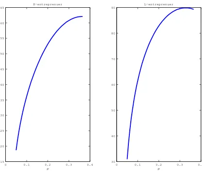
[Insert Figure 5]

Figure 5 shows the difference of ex-ante welfare for them between bubble and bubbleless economies and indicates the appearance of a bubble is welfare-improving for both types of entrepreneurs. Intuitively, this comes from the difference in the rates of return. Without bubbles, L-entrepreneurs end up with accumulating their wealth through a low return savings vehicle with a rate of return of αL

/u′σ

t . On the other hand, a bubble provides a high

rate of return vehicle for them, Pt+1/Pt. This increase in the rate of return

contributes to improving the net worth of entrepreneurs and their welfare.

4

Conclusion

We examined the effect of asset price bubbles in the Kiyotaki-Moore model. We have shown that the dynamic interactions between bubble-asset price, land price, and output generate powerful bubbly dynamics. The boom-bust cycles in bubble-asset price cause boom-crash cycles in the land market si-multaneously, like a contagion by affecting the fundamentals of land. We also numerically analyzed the welfare effects of bubbles in transitional dynamics. We have found that bubbles tend to be welfare-improving.

References

[1] Aoki, Kosuke, and Kalin Nikolov. 2011. “Bubbles, Banks and Financial Stability,” Working Paper, CARF-F-253, The University of Tokyo.

[2] Bernanke, Ben, and Mark Gertler. 1989. “Agency Costs, Net Worth, and Business Fluctuations,” American Economic Review, 79(1): 14–31.

[3] Bernanke, Ben, Mark Gerlter, and Simon Gilchrist. 1999. “The Financial Accelerator in a Quantitative Business Cycle Framework,” in J. Taylor and M. Woodford eds, the Handbook of Macroeconomics, 1341-1393. Amsterdam: North-Holland.

[4] Brunnermeier, Markus. 2009. “Deciphering the Liquidity and Credit Crunch 2007-2008.,” Journal of Economic Perspectives, 23(1): 77-100.

[5] Farhi, Emmanuel, and Jean Tirole. 2011. “Bubbly Liquidity,” forthcom-ing in Review of Economic Studies.

[6] Grossman, Gene, and Noriyuki Yanagawa. 1993. “Asset Bubbles and Endogenous growth,” Journal of Monetary Economics, 31(1): 3-19.

[7] Hellwig, Christian, and Guido Lorenzoni. 2009. “Bubbles and Self-Enforcing Debt,” Econometrica, 77(4): 1137-1164.

[8] Hirano, Tomohiro, and Noriyuki Yanagawa. 2010a. “Asset Bubbles, En-dogenous Growth, and Financial Frictions,” Working Paper, CARF-F-223, The University of Tokyo.

[9] Hirano, Tomohiro, and Noriyuki Yanagawa. 2010b. “Financial Insti-tution, Asset Bubbles and Economic Performance,” Working Paper, CARF-F-234, The University of Tokyo.

[10] Holmstrom, Bengt, and Jean Tirole. 1998. “Private and Public Supply of Liquidity,” Journal of Political Economy, 106(1): 1-40.

[11] Kiyotaki, Nobuhiro, 1998. “Credit and Business Cycles,” The Japanese Economic Review, 49(1): 18–35.

[13] Kocherlakota, R. Narayana. 1992. “Bubbles and Constraints on Debt Accumulation,” Journal of Economic Theory, 57(1): 245-256.

[14] Kocherlakota, R. Narayana. 2009. “Bursting Bubbles: Consequences and Cures,” University of Minnesota.

[15] Martin, Alberto, and Jaume Ventura. 2010. “Economic Growth with Bubbles,” Universitat Pompeu Fabra.

[16] Martin, Albert, and Jaume Ventura. 2011. “Theoretical Notes on Bub-bles and the Current Crisis,” IMF Economic Review, 59(11): 6-40.

[17] Matsuyama, Kiminori. 2007. “Credit Traps and Credit Cycles,” Amer-ican Economic Review, 97(1): 503-516.

[18] Miao, Jianjun, and Pengfei Wang. 2011. “Bubbles and Credit Con-straints,” mimeo, Boston University.

[19] Miller, Marcus, and Joseph Stiglitz. 2010. “Leverage and Asset Bub-bles: Averting Armageddon with Chapter 11?,” The Economic Journal, 120(544): 500-518.

[20] Santos, S. Manuel, and Michael Woodford. 1997. “Rational Asset Pricing Bubbles,” Econometrica, 65(1): 19-58.

[21] Sakuragawa, Masaya. 2012. “Savings and Bubbles,” mimeo, Keio Uni-versity.

[22] Tirole, Jean. 1982. “On the Possibility of Speculation under Rational Expectations,” Econometrica, 50(5): 1163-1182.

[23] Tirole, Jean. 1985. “Asset Bubbles and Overlapping Generations,” Econometrica, 53(6): 1499-1528.

[24] Ueda, Kazuo. 2011. “Japan’s Deleveraging since the 1990s and the Bank of Japan’s Monetary Policy: Some Comparisons with the U.S. Experi-ence Since 2007,” Working Paper No. CARF-F-259, The University of Tokyo.

Output

Networth

Land Bubble Demand

prie

prie for assets

Output

Net worth

Land Bubble Demand

prie

prie forassets

Output

Networth

Land Bubble Demand

prie

prie for assets

Y t t+1

Bubble eonomy

Bubbleless eonomy

Y

bubbl e Y

bubbl el ess

0 20 40 60 80 0

5 10 15 20 25 30 35

t

Bubble price (P )

0 20 40 60 80

2 2.2 2.4 2.6 2.8 3 3.2

t

Land price (q )

0 20 40 60 80

0.9 0.95 1 1.05 1.1

t

Interest rate (r )

0 20 40 60 80

1.6 1.7 1.8 1.9 2 2.1 2.2

t Output (Y )

0 20 40 60 80

0.05 0.1 0.15 0.2 0.25 0.3 0.35

t

Consumption (C )

0 20 40 60 80

1 1.1 1.2 1.3 1.4 1.5

t

Intermediate goods (Z )

0 0.1 0.2 0.3 0.4 116

118 120 122 124 126 128 130 132 134

H−entreprenuer in bubble economy

p

0 0.1 0.2 0.3 0.4 115

120 125 130 135 140

L−entreprenuer in bubble economy

p

0 0.1 0.2 0.3 0.4 50

60 70 80 90 100 110

H−entreprenuer in bubbleless economy

p

0 0.1 0.2 0.3 0.4 30

40 50 60 70 80 90

L−entreprenuer in bubbleless economy

p

0 0.1 0.2 0.3 0.4 15

20 25 30 35 40 45 50 55 60 65

H−entreprenuer

p

0 0.1 0.2 0.3 0.4 30

40 50 60 70 80 90

L−entreprenuer

p

Appendices

A

Proof of Proposition 1

In the steady-state bubble economy, from (23), uσ

is

uσ

= α

H

pβ

1−β+pβ. (B1)

By substituting (B1) into (24), we can derive (26).

B

Proof of Proposition 2

In order to prove Proposition 2, we first characterize an equilibrium of the bubbleless economy. When there is no bubble, the interest rate, user cost, output, and wealth evolve over time as, respectively,

r′ t=

αL

u′σ t

, (A1)

qt=ut+

uσ t

αLqt+1(1−γ) (A2)

Y′ t+1 =

αH

σ (u

′ t)

1−σ

K′H t +

αL

σ (u

′ t)

1−σ

K′L

t , (A3)

A′ t+1 =

αH

u′σ t

βpA′ t+

αL

u′σ t

β(1−p)A′

t. (A4)

In the bubbleless economy, the interest rate equals the rate of return of L-projects, so even L-entrepreneurs end up producing in equilibrium, which means that K′L

≥0 and Z′L

≥0.

Given an initial condition, Y0, and Pt = 0 for all t ≥0, the perfect

fore-sight equilibrium path of the bubbleless economy is described by sequences

{qt, At, rt, ut, Yt} ∞

t=o, satisfying (10), (22), and (A1)-(A4).

In the steady-state, the user cost is

Condition (26) is equivalent to

uσ

≥u′σ

. (A6)

This means that as long as bubbles can exist, the user cost in the steady-state bubble economy is greater than that in the steady-state bubbleless economy.

Sinceuσ

≥u′σ

and KH

≥K′H

,from (20) and (A3),

Y ≥Y′

. (A7)

Moreover, uσ

≥u′σ

and KH

≥K′H

mean

uKH

σ ≥ u′

K′H

σ . (A8)

Hence,

ZH

≥Z′H

, (A9)

A≥A′

, (A10)

because in equilibrium, uKH

/σ =ZH

/1−σ =βpAandu′

K′H

/σ=Z′H

/1−

σ =βpA′

hold.

We also know that aggregate consumption is a fraction 1− β of the aggregate wealth. Hence,

C ≥C′

. (A11)

Aggregate TFP can be defined as

TFP≡ Y

(K σ

)σ( Z

1−σ

)1−σ, TFP

′

≡ Y

′

(K′

σ

)σ( Z′

1−σ

)1−σ, (A12)

where Z =ZH

+ZL

and Z′

=Z′H

+Z′L

. Hence,

TFP =αH ≥TFP′

≡ α

H

Z′H

−αL

Z′L

Z′ . (A13)

C

Proof of Proposition 3

By substituting (18), (22), and (23) into (21), we obtain

φt =σp+

δ−φt

δ−φt+1

where φt ≡qt/βAt.

Given a state variable Yt, there is a unique price path {qt, Pt} ∞

t=0 where

φt becomes constant over time and satisfies

φ=σp/γ. (C2)

Once φt becomes constant, then we can derive (28)-(30) from (22) and (C2).

Using (18), (20) can be rewritten as

Yt+1 =

αH

σ (σβpAt)

1−σ

. (C3)

(C3) can be rearranged as (27) using (28), (29), and the definition of At.

Hence, the economy converges to the steadystate according to (27), and (28)-(30). The initial values of {q0, P0} are determined so that the economy