The Role of Consumption Labor Complementarity as a Source of Macroeconomic Instability

Munich Personal RePEc Archive

The Role of Consumption-Labor

Complementarity as a Source of

Macroeconomic Instability

Gliksberg, Baruch

University of Haifa

June 2010

Online at

https://mpra.ub.uni-muenchen.de/24816/

The Role of Consumption-Labor Complementarity as a

Source of Macroeconomic Instability

Baruch Gliksberg

University of Haifa

June, 2010

The equilibrium ramification of a balanced budget rule are scrutinized in a one sector

growth model augmented with investment frictions and a non-separable utility function

in consumption and leisure. Edgeworth-complementarity between consumption and

labor is formulated so as to generate a positive co-movement of consumption, output,

and hours worked, as found in the data. Calibration of the model to the U.S. economy

provides evidence that a balanced budget rule with a Taylor type monetary policy

induce determinate equilibria.

JEL Classification: C62, C63, E4, E52, E61, E62, E63.

Keywords: Fiscal-Monetary policy; Non-Separable Utility; Consumption-Labor

Complementarity; Endogenous Labor; Stabilization; Determinacy; Investment;

1. Introduction

It seems plausible that versions of business cycle models that exhibit a positive

co-movement between consumption and labor may also exhibit indeterminacies. A

noteable attempt to link between indeterminacies and the positive co-movement

between consumption and labor is found in Benhabib and Wen (2004). They show that

under indeterminacy, aggregate demand shocks are able to explain not only aspects of

actual fluctuations that standard RBC models predict fairly well, but also aspects of

actual fluctuations that standard RBC models cannot explain, such as the hump-shaped,

trend reverting impulse responses to transitory shocks found in US output [Cogley and

Nason (1995)] the large forecastable movements and comovements of output,

consumption and hours [Rotemberg and Woodford (1996)] and the fact that

consumption appears to lead output and investment over the business cycle.

Indeterminacy arises in their model due to capacity utilization and mild increasing

returns to scale. Subsequent literature, such as Linnemann (2008) and Meng and Yip

(2008), contributes to this literature by improving our intuition as to the causes of

indeterminacy.

In Linnemann (2008), equilibrium indeterminacy can arise in a neoclassical growth

model when the government continuously balances its budget through adjustments of

the income tax rate1. Linnemann (2008) puts emphasis on a steady state in which

leisure is constant although consumption may grow. In this case, complementarity

between consumption and employment emerges as a stabilizing mechanism. Meng and

Yip (2008) relax the restrictions commonly imposed on the magnitude of capital

externalities in one-sector models with Cobb-Douglas technology. They find that

indeterminacy can arise either if utility is separable in consumption and leisure and

1

there are negative capital externalities; or: utility is non-separable and the social

elasticity of production with respect to capital is greater than one. In addition, with

Cobb-Douglas technology they show that leisure must be a normal good for

indeterminacy to occur [that is, the presence of income effects on the demand for

leisure is a necessary condition for indeterminacy]. There is no restriction in meng and

Yip (2008) analysis on whether consumption and labor are complements or substitutes.

At this time the literature provide no clue as to the direction of causality where

equilibrium is indeterminate and consumption co-moves with labor, so it remains a

matter of faith. Either, as in Benhabib and Wen (2004) under indeterminacy, aggregate

demand shocks explain the large forecastable movements and comovements of output,

consumption and hours, or , complementarities between consumption and labor are

responsible both to indeterminacies a-la Benhabib and Wen (2004) and to the positive

co-movement found in the data. It should be noted however, that the assumption of

additive separability of utilities with respect to consumption and leisure has been

typically made more for convenience than from conviction. Basu and Kimball (2002)

and Kimball and Shapiro (2008) reject additive separability and arrive at the view that

the utility function exhibits complementarity between consumption and labor by

considering facts about lung-run labor supply. Hall (2008) and Raj (2006) also share

this view. Their view also points to predictions in the context of Benhabib and Wen

(2004). For example, complementarity between consumption and labor provide a

straightforward channel for monetary policy to cause an increase in output. When labor

and consumption are complementary, the increase in consumption is enough to cause

output to increase as long as interest and wealth effects are not too large.

Note that in most RBC models it is implicit that the government seeks to stabilize

fluctoations due to self fulfillinf expectations. In such a case, consumption-labor

complementarity can overturn policy outcomes.

This paper puts emphasis on characterizing policy rules that potentially subdue the

self fulfilling fluctutions that come to pass from the complementarity between

consumption and hours worked. It maintains, however, the assumption that the

consolidated government operates a balanced budget. In simple settings the conditions

under which monetary policy can lead to indeterminacy under a balanced budget

requirement are well understood: active interest rules within a balanced budget

requirement generate determinacy and passive rules generate indeterminacy. Prominent

papers in this literature include Benhabib et. al. (2001) [who discuss monetary policy

rules where money and consumption are Edgeworth complements and the policy

affects households allocation at the private level between financial assets and capital

assets via an arbitrage channel] and Huang and Meng (2007) [who consider an effect of

policy on households via the arbitrage channel and an effect on firms via a pricing

channel in a model with monopolistic competition and nominal price rigidity]. This

paper contributes to existing literature by considering an additional channel: a labor

channel, where consumption and labor are assumed Edgeworth complements.

Accordingly, it is assumed throughout that the utility function is non-separable in

consumption and leisure and, in line with Hall (2008), that consumption and labor are

complements. The upshot of this paper is that controlling the real rate of interest is a

necessary condition for the determination of expectations. The model calibrated to the

U.S economy provides evidence that: a) operating an interest rate rule such that the

expected real rate of interest is above its steady state level during booms and below its

operating an interest rate rule such that the expected real rate of interest is constant at

all times is sufficient to induce equilibrium determinacy; c) a non-monetary version of

the model is expected to exhibit indeterminacies as demonstrated in Meng and Yip

(2008)2.

The rest of the paper is organized as follows: section 2 illustrates a model with

endogenous labor-leisure choice where consumption and labor are Edgeworth

complements. This model is extended to include a concave investment technology and

a cash-in-advance constraint. The cash-in-advance constraint is introduced so as to

mimic the role of complementarity between consumption and money. Section 3

contains local stability analysis with the least amount of restrictions over the functional

forms of utilities and production technology. In section 4 long run elasticities and deep

structural parameters are calibrated to the U.S. economy. Results show that for a

plausible range of parameters, under a requirement that the consolidated budget is

balanced throughout, local-real-determinacy is ensured where monetary policy is

neutral or active. Section 5 concludes.

2

2. A Model with Endogenous Labor-Leisure Choice and Frictions in Investment

It is assumed throughout the paper that the consolidated government runs a balanced

budget within which the central bank operates an interest rate feedback rule. Dupor

(2001) and Benhabib et al. (2001) discuss the issue of local real determinacy in a

continuous time model where the monetary authority sets a nominal interest rate as a

function of the instantaneous rate of inflation. The policy considered here follows this

line and is also in one line with the forward-looking policy considered by

Schmitt-Grohé and Uribe (2007) and Carlstrom and Fuerst (2005) in their discrete-time

models3.

Money enters the economy via a cash-in-advance constraint on consumption.

Following Benhabib et. al (2002), and to avoid steady state multiplicity, attention is

restricted to equilibria with a strictly positive nominal interest rate. This approach

receives substantial support in Schmitt-Grohé and Uribe (2007)4. Finally, to keep the

focus on labor channel effects and to abstract from cost-channel effects it is assumed

throughout that nominal prices are flexible and that markets are perfectly competitive.

2.1. The Economic Environment

Households – The model is a continuous time, flexible price version of

Schmitt-Grohé and Uribe (2007) with endogenous labor-leisure choice and endogenous

investment. The economy is populated by a continuum of identical infinitely long-lived

3

As we know, the instantaneous rate of inflation in a continuous-time setting is the right-derivative of the logged price level and thus, the discret-time counterpart of a countinuous-time policy rule that sets the interest rate in response to the instanteneous rate of inflation is characterized by forward-looking policy that responds to expected future inflation.

4

households, with measure one. The representative household’s lifetime utility is given

by

dt L c u e

U t

) 1 , ( 0

− =

_∫

∞ −ρ

where ρ>0 denotes the rate of time preference, c denotes consumption. It is assumed

that households are endowed with one unit of leisure. L and l =1− Ldenote labor and

leisure, respectively. u(c,l) is twice differentiable, strictly increasing in both arguments

and concave where consumption and leisure are Edgeworth substitutes ( ucl<0). We

also assume that ucc-ucluc/ul<0 and ull-uclul/uc<0 which implies that consumption and

leisure are normal goods. Apart from being plausible, this assumption is imperative in

order to give rise to indeterminacies a-la Meng and Yip (2008).

It is also assumed that consumption and money balances are Edgeworth complements.

To keep the analysis simple and tractable while maintaining the consumption-money

complementarity assumption, money enters the economy via a cash-in-advance

constraint on consumption5. In addition to money, households can store wealth in

government-issued non-indexed bonds and physical capital. Bonds pay a net nominal

interest of R>0. Capital is either utilized for production or consumed paying an

adjustment cost. The household’s budget constraint is therefore described as:

τ

π

π − + −

− = + +

+I b m (R )b m f(k,L) c

where I is the flow of investment, b is the real value of government bonds, m is the real

value of money balances, k is the stock of capital, τ is a real lump-sum tax and π is the

rate of inflation. Note that all variables are time-dependent (the time argument is

5

omitted to keep notation simple). Finally it is assumed that the function, f(k,L), is twice

differentiable, strictly increasing and displays a constant returns to scale production

technology. We further assume that factor markets are competitive, thus, production

factors are paid their marginal product. By defining a≡b+m as the real value of

non-capital wealth the household’s budget constraint becomes:

τ

π − + + − − − −

= R a Rm rk wL c I

a ( )

Where r and w denote capital rent and labor compensation, respectively. The

household’s consumption is then subject to the cash-in-advance constraint

∫

+

≤ =

T t

t

m ds s c T

F( ) ( ) . Normalizing T to 1 the CIA constraint can be approximated as:6

Finally, assuming that the stock of capital depreciates at a rate δ, the household’s

lifetime maximization problem becomes

m c

k I k

I c wL rk Rm a R a

t s

dt L c u e Max t

≤

− =

− − − + + − − =

−

∫

∞ −

δ

ϕ

τ

π

ρ

) (

) (

. .

) 1 , ( 0

With the following no-Ponzi-game condition

and where

ϕ

(I) is increasing and concave with

ϕ

(0)=0. This specification suggests that

6

This version of CIA is similar to Rebelo andXie (1999). Formally, the cash-in-advance constraint is

∫

+

≤ =

T t

t

m ds s c T

F( ) ( ) . A Taylor series expansion gives = + T ( )+ 2

1 ) ( T )

(T c t 2c t

F and so (4)

can be interpreted as a first-order approximation. Finally, and without loss of generality to subsequent analysis, T is normalized to 1.

m

c≤

0

0 + =

∫ −π −

∞

→ e [a(t) k(t)]

Lim t

adjustments to the stock of capital are costly and that adjustment costs are increasing

with investment and convex7.

The household chooses sequences of {c,I,L,m} so as to maximize its lifetime utility,

taking as given the initial stock of capital k(0), and the time paths of τ,R, and π.

An optimal program must choose c,m,L and I so as to maximize the

current-value Hamiltonian

[

(

)

] [

(

)

]

(

)

)

1

,

(

1

u

c

L

R

a

Rm

rk

wL

c

I

I

k

m

c

H

≡

−

+

λ

−

π

−

+

+

−

−

−

τ

+

ϕ

−

δ

+

ξ

−

Thus,

the necessary conditions for an interior maximum of the household’s problem are

ξ

λ

+

= − ) 1 ,

(c L

u_c

) ( '

1 I

ϕ

λ

=

λ

) 1 , (c L u

w₌ l −

R

λ ξ =

ξ

≥

0

;

ξ

(

m

−

c

)

=

0

Where λt and t (in the current-value Hamiltonian the time subscripts are omitted to

simplify notation) are co-state variables interpreted as the marginal valuation of a unit

of financial assets and installed capital, respectively, and ξt is a Lagrange multiplier

associated with the CIA constraint.

Second, the co-state variables must evolve according to the law

7

]

[ + −R

=

λ

ρ

π

λ

δ ρ λ +( + ) −

= r

Since attention is restricted to steady states with non negative inflation targets, the

nominal rate of interest is positive near the steady state. As a result, equation (8)

implies that ξ, the Lagrange multiplier associated with the cash-in-advance constraint

in non zero. It then follows from (9) that m=c and from (8) and (5) that

) 1 ( ) 1 ,

(c L R

u_c − =

λ

+ . The interpretation is simple: near a steady state with positive

nominal interest rate holding money entails opportunity costs. Thus, equilibrium

amount of (real) money that minimizes the opportunity cost associated with money

holding while still satisfying condition (4) is m=c. Accordingly, the law of motion for

the real value of financial assets becomes

a =(R−π)a+rk + wL −c(1+R)−I −τ

and the law of motion for capital is

k I

k =ϕ( )−δ

We study equilibria close to the steady state and we assume that fiscal policy is passive

[according to Leeper (1991)], therefore, the transversality condition holds.

Let η denote the ratio between the two co-state variables, . Accordingly,

, and thus, substituting in equations (10) - (11) and rearranging yields the

evolution of η:

η

=−fk(k,L)+

η

(R−

π

+

δ

)

Equations (10), (13) – (14) fully describe the optimal instantaneous decision of the

representative household as it takes the time paths of τ, R, and π as given.

λ η≡

λ λ η λ

The Government

Following Benhabib et. al. (2001) it is assumed that monetary policy takes the form of

an interest-rate feedback rule whereby the nominal interest rate is set as an increasing

function of instantaneous inflation. Specifically, it is assumed that

) (π R

R=

Where R(π) is continuous, non-decreasing and strictly positive, and there exists a

steady-state,(π*), where π* >−ρ such that R(π*)= ρ+π*. It is further assumed that the

monetary authority reacts to an increase in the rate of inflation by increasing the nominal

rate of interest. That is, ( >0 ∂

∂

)

π

R *

π . Following the terminology of Leeper (1991), the

government operates under a passive fiscal policy and levy lump-sum taxs. It is assumed

that government disbursements include purchases and interest payments over the

outstanding debt. Thus, the consolidated government’s nominal budget constraint is

Pg+RB=M +B+P

τ

where B and M denote nominal stocks of bonds and money, respectively, P is the level

of nominal prices, and g denotes government purchases. The central bank imposes the

desired interest rate by controlling the price of riskless nominal bonds and exchanging

money for bonds at any quantities demanded at that price. In that sense, the nominal rate

of interest is exogenous and the M and B are endogenous. Simple algebraic

manipulations of equation (16) yield that a≡m+b evolves according to:

) ( )

(R a Rm g

a= −π − − τ −

Equilibrium – In equilibrium, the goods market, the factors market and the assets

describe a rational expectations equilibrium given the time paths of τ, R, and π as

(exogenously) given. Thus, our discussion will focus on whether the representative

agent can construct an isolated equilibrium trajectory in the (λ,η,k) space given a

predetermined level of k and a common knowledge with respect to the stance of

monetary policy.

Conjecture that an isolated equilibrium exists. Then, equations (18), (19) and (20)

describe instantaneous equilibrium in the goods market, labor market and the assets

market respectively:

) 18 (

g k I k c k L k

f( , (λ,η, ))= (λ,η, )+ (λ,η, )+

) 19 (

λ

η

λ

η

λ

η

λ

, , )) ( ( , , ),1 ( , , ))

( ,

(k L k u c k L k

f l

L

− =

) 20 (

)) , , ( ( 1

)) , , ( 1 ), , , ( (

k R

k L k c u_c

η λ π

η λ η

λ λ

+

− =

also, Equation (6) demonstrates that the rate of investment depends only on η . Thus,

) ( )

( '

1

η

ϕ

η

I I

I ⇒ =

=

2.2. Equilibrium Dynamics

Partially deriving equations (18)-(20) with respect to λ,η and k [appendix A.1] yields

(

)

) 1 , ( ) 1 , ( ) , ( ) 1 , ( ) , ( ) , ( ) 1 , ( ) 1 , ( ) , ( ) ( '' ) 1 , ( ) 1 , ( ) 1 , ( ) , ( ) ( )) 1 , ( ) 1 , ( ( ) 1 , ( ) , ( ) ( )) 1 , ( ) 1 , ( ( ) 1 , ( ) ( '' 1 ) ( )) 1 , ( ) 1 , ( ( 1 ; ) , ( , ) ( '' 1 , , ) ( '' 1 2 2 2 2 L c u L c wu L k f L c u L k f L k f L L c u L c wu L k f I L c u L L c u L c wu L k f w L R L c u L c wu L L c u L k f R L c u L c wu L L c u I R L c u L c wu L R L w L k f c I L w c L w c I I ll cl LL cl k kL k ll cl LL cl ll cl LL cl cc k cc k k cl cc cc cl cc k k k − + − − − + − = − + − − − = − + − − − = − + − − − − = − + − − − − = − + − − + + − = + = − = = − =

λ

λ

λ

ϕ

η

λ

π

λ

π

π

λ

ϕ

η

π

π

λ

π

ϕ

η

ϕ

η

η λ π π η η π λ λ η η λ λ η

Thus, the dynamics of all the variables in the economy can be described by (λ,η,k)

which evolve according to:

[

π

λ

η

π

λ

η

]

λ

η

π

λ

η

λ

η

τ

η

λ

η

λ

η

η

λ

λ

− − − = = = = ) , , ( ) , , ( ) , , ( , , ) , , ( ) , , ( ) , , ( ) , , ( k m k) ( R k a k) ( k) ( R a k H k k G k F where )] , , ( ) , , ( [ ) , ,

( k k R ( k)

F λ η ≡λ ρ+π λ η − πλ η

] ) , , ( ) , , ( [ ) , , , ( ) , ,

(

λ

η

k ≡−f k L(

λ

η

k) +

η

R

π

(

λ

η

k) −

π

λ

η

k +

δ

G _k

k I

k

H(λ,η, )≡ϕ( (η))−δ

and where the transversality condition is −₀∫[ ( , , )− ( , , )] [ ( , , )₊ ]₌0 ∞

→ e a k k

Lim t ds k k) ( R

t

λ

η

3. Equilibrium and Local Real Determinacy

Linear models with infinite horizon generally admit infinitely many rational

expectations solutions. Consequently, some selection devices are needed to narrow the

set of applicable solutions. This paper emphasizes a selection device according to

Evans and Guesnerie (2005) who show that the saddle-path solution is bound to be

selected from a multiple of applicable solutions.

Definition - Equilibrium displays Local-Real-Determinacy (LRD) if there exists a

Saddle-Path stable solution in the(λ,η,k)space.8 Otherwise equilibrium displays

Non-LRD.

Local Real Determinacy

Equations (5), (7), (23)–(25) imply that in the steady state _R(

π

*₎₌

ρ

₊

π

*_,

δ

ρ

η

π

ρ

λ

+ = + + − = , ( , ) 1 ) 1 , ( * * * * * *

* uc c L fk k L

,

ϕ

(I(

η

*))=

δ

k*, _*

* *

* ( ,1 )

λ

L c u

w ₌ l −

[asterisk

throughout denote steady state levels]. Also, a linear approximation of the dynamic

system near the steady state (

λ

*,

η

*,_k*) _{is obtained through the system}





































− − −                   − − − + − − − + − + − + − − − − − − − = * * * ) ( '' ) ( ' 0 ) 1 ( ) 1 ( ) 1 ( ) 1 ( ) 1 ( ) 1 ( 2 * * * * * * * * * * * * * * * * * * * * * * * * * * * * k k X A I I R L f f R L f R L f R R R k k k kL kk kL kL k η η λ λ δ η ϕ ϕ π η π η δ ρ π η π λ π λ π λ η λ π η π η λ π λ π η π λ π

where A is the Jacobian of equations (23)-(25) andR_π* denotes

π π

∂ ∂R( )

at π*.

8

The solution of the characteristic equation of A depends on R_π* that exhibits the stance

of monetary policy near the steady state. Note that

)

1

,

(

)

1

,

(

ˆ

1

)

1

(

)

(

* * * * * * 2 * * * * * * * * * * * * * * * 2 * * * * * 2 * * * * * * * * * * * * * * * 3 2 1 ) ( ' ' ) ( ' 0 * * ) ( ' ' 1 * 1 ) ( ' ' ) ( ' 0

L

c

u

L

c

u

w

where

B

Det

R

R

B

Det

R

A

Det

cl cc k kL kk kL kL k cc k cc k kL kk kL kL k I I L f f L f L f L u f L u I L R I I L f f L f L f

−

+

−

−

≡

−

−

=

−

−

=

=

                    − − − − − + − − − − + −                   − − − − − + − δ η ϕ ϕ δ ρ η ϕ δ η ϕ ϕ δ ρ π π π η λ η λ π π η λ η λ π

λ

θ

θ

θ

And that * * * * * * * 3 2

1

θ

θ

( ) ( π 1)(

η

π

η

λ

π

λ)

ρ

η

θ

+ + =Trace A = R − − + − f_kLL

Where

θ

_i

,

i

=

1

,

2

,

3

denote the eigenvalues of A. Thus, with one predetermined variable,

a necessary condition for LRD is that _*

1

(

ˆ

)

0

* 3 2 1

<

−

−

=

Det

B

4. Solution, Calibration, and Computation

According to equations (5) and (7) the shadow real wage as seen by the household is

) 1 ( ) 1 , ( ) 1 , ( ) , ( R L c u L c u L c w c l ₊ − − = .

Define the elasticity of the wage with respect to consumption when labor is held

constant as

c cc l cl u u c u u c c L c w L

c = −

∂ ∂ ≡ ) ln( )) , ( ln( ) , (

ζ

and the elasticity of intertemporal

substitution for consumption s(c,L)and the consumption-constant elasticity of labor

supply h(c,L) by

c cc u u c L c

s( , ) ≡− 1 and c cl l ll u u L u u L L L c w L c

h ∂ =− +

∂ ≡ ) ln( )) , ( ln( ) , ( 1 .

Finally define (1 )

) 1 , ( ) 1 , ( ) , ( ) , ( R L c u L c u c L c L L c w L c c l ₊ − − = ≡

ω

and note that

R L c u_c + − = 1 ) 1 , (

λ

Since the Hessian _

     ll cl cl cc u u u u

is symmetric, the three elasticities,

ζ

(c,L) s(c,L)and

) , (c L

h , plus ω(c,L)and λ determine all local first and second derivatives of the

function u(c,1−L)apart from overall scale of felicity which has no economic meaning.

Accordingly, simple algebra obtains

(

)

(

)

      + − + − = − = + − = = + = * * * * * * * * * * * * * * * * * * * * * * * * * * * * * ) 1 ( 1 ; 1 ; ) 1 ( ; ); 1 ( s R s h L w u s c s w u s c R u w u R u ll cl cc l c

λ

ζ

ω

λ

λ

ζ

λ

λ

λ

where asterisk denote steady state levels9. A similar exercise obtains that

2 * * * * * * * 2 * * * * * * * * ; ; ; ) 1 ( ; 1 ) 1 ( L c f L k c f k c f k c f c

I _{k kk} αω _kL αω _LL αω

α αω α ω α − = = − = − = − − + = 9

(proof in appendix A.2) and

(

)

2 2 * 2 * * * * * * * ) 1 ( ) 1 )( 1 ( ) 1 ( ) 1 ( 2 ) ( ' ' ; ) )( 1 ( ) ( ' ; ) ( − + − − + − − − − = + − = = ω α αω ω α δ ω α ρ α ϕ αω δ ρ α ϕ δ ϕ c k I c k I k I

(proof in appendix A.3)

Where α,δ,ρ,ω,ζ,h,s are obtained from estimates of stationary time series.10

,

At this point, finding the restrictions on monetary policy so as to induce LRD is straight

forward: First, steady state levels uc*,ul*,ucc*,ucl*,ull*,

* * * * * , , ,

, f_k f_kk f_kL f_LL

I , ) ( ' ' ), ( ' ),

(I* ϕ I* ϕ I*

ϕ are substituted into equation (22) to obtain

* * * * * * * * * * , , , , , ,

, λ η λ _η

π

_λ

π

_η

π

η c c ck L L Lk k

I that depend only on the long run estimate of

α,δ,ρ,ω,ζ,h,s . Then, steady state levels

) ( '' , , , , , , , , * * * * * * * * * * * _I L L L c c c

Iη λ η k λ η k

π

λ

π

η

π

k

ϕ

are substituted into the Jacobian

[image:18.595.94.533.514.645.2]

matrix A.

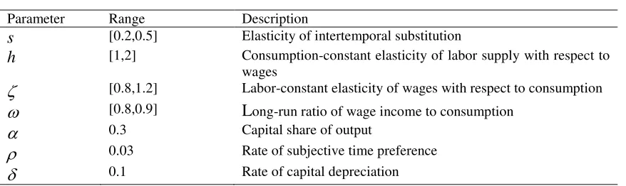
Table 1 – Structural Parameters and Elasticities

Parameter Range Description

s [0.2,0.5] Elasticity of intertemporal substitution

h [1,2] Consumption-constant elasticity of labor supply with respect to wages

ζ

[0.8,1.2] Labor-constant elasticity of wages with respect to consumption

ω

[0.8,0.9] _{Long-run ratio of wage income to consumption}

α

0.3 Capital share of output

ρ

0.03 Rate of subjective time preference

δ

0.1 Rate of capital depreciation

10_ϕ''(I)<0

. Thus, the values of α,δ,ρ,ω should be calibrated so as to ensure that ϕ''(I) is negative at the steady-state investment. Specifically,

αδ δ ρ δ ρ α ω ϕ − + + − < ⇔

<0 (1 )( )

) ( '

' I*

According to the theory, ω equals labor income divided by consumption expenditure.

Taking nominal wages and salaries from the U.S National Income Accounts and

dividing by nominal spending on non-durable consumption and services gives an

average ratio of 0.9. Basu and Kimball (2002) use the prices as perceived by consumer

so they define ω using after-tax wage. Thus they use

ω=0.8 as their preferred value. It

should be noted however, that in the present context, results are robust to

ω as long as

αδ δ ρ

δ ρ α ω

− +

+ −

<(1 )( ) which is essential to ensure that the investment technology is

concave. For that matter, and given the assumed values of α,ρ,δ, ω must be less than

0.91.

For all values specified in Table 1 Det(Bˆ)>0 which imply that the Taylor principle is

necessary to ensure local real determinacy. Furthermore, the upshot of explicitly

solving the characteristic equation of A for values of Table 1 is that an active policy

stance, R_π* >1, induces two unstable eigenvalues and one stable eigenvalue and hence

local-real-determinacy. A neutral policy stance, R_π* =1, brings about one stable

eigenvalue, one zero eigenvalue and one unstable eigenvalue and hence

local-real-determinacy. A passive policy stance, R_π* <1, brings about two stable eigenvalues and

one unstable eigenvalue and hence equilibrium is Non-LRD11.

11

5. Conclusion

This paper considers local real determinacy (LRD) as a prerequisite for

macroeconomic stability. LRD was examined under a simple forward-looking interest

rate feedback rule and a passive fiscal-policy with non distorting taxation where both

labor supply and investment are endogenous. The focus is on labor market dynamics

that derive from complementarities between consumption and hours worked. The

model is specified so as to apply for a wide range of utilities through transformation

from ethereal expressions to long run elasticities.

The model gives rise to a labor market channel. This channel of monetary

policy, in an economy calibrated to the US economy, was found to act together with the

arbitrage channel of monetary policy. The Taylor principle is shown to induce LRD.

Furthermore, a neutral policy stance, such that the expected real rate of interest is

Appendix A A.1 L L c u c L c u L L k f L k f L L c u c L c u L L k f L L c u c L c u w L L k f R L L c u c L c u R L L c u c L c u R L L c u c L c u R c L w L k f I c L w c L w I I k ll k cl k LL kk ll cl LL ll cl LL k k cl k cc cl cc cl cc k k k ) 1 , ( ) 1 , ( ) ) , ( ) , ( ( ) 1 , ( ) 1 , ( ) , ( ) 1 , ( ) 1 , ( ) , ( ) ( ) 1 , ( ) 1 , ( ) ( ) 1 , ( ) 1 , ( ) ( ) 1 , ( ) 1 , ( 1 ) , ( ) ( '' 1 2 − − − = + − − − = − − − + − = = − − − = − − − − − − − = + = + + = = − =

λ

λ

λ

π

π

λ

π

π

λ

π

π

λ

ϕ

η

η η η λ λ λ π η π η η λ π λ λ η η η λ λ η A.2

It is assumed throughout that a large number of firms, each of which produces a

homogenous commodity using a constant returns-to-scale production-technology,

operate in a competitive setup of markets for goods and factors. Accordingly,

L L k f k L k f L k

f( , )= _k( , ) + _L( , ) . And, the capital share of output is

α

Taking partial derivatives of both sides of f(k,L)= f_k(k,L)k+ f_L(k,L)L and

assuming the market clearing conditions for goods and factor markets, we obtain a set

of equations I c L k f k L L k f L k f L L c w L k f k L k f L k f L k f k L k f L L c w k L k f L k f LL kL LL k kk k k + = − = − = − − = = + = ) , ( ) , ( ) , ( ) , ( ) , ( ) , ( ) 1 ( ) , ( ) , ( ) , ( ) , ( ) , ( ) , (

α

α

α

Of which the solutions with respect to I and the partial derivatives of f are

2 * * * * * * * 2 * * * * * * * * ; ; ; ) 1 ( ; 1 ) 1 ( L c f L k c f k c f k c f c

I _{k kk} αω _kL αω _LL αω

α αω α

ω

α _{=− = =−}

− = −

− +

= where

* * * c L w ≡

ω

and asterisk denote steady state levels

A.3

A second order Taylor expansion of the investment technology ϕ(I):

2 * * * * * ) )( ( ' ' 2 1 ) )( ( ' ) ( )

(I =ϕ I +ϕ I I −I + ϕ I I −I

ϕ Specifically it is used to approximate

ϕ(0)=0.

Rearranging the Taylor expansion for

ϕ(0)=0

implies that

2 * * * * * '( ) ( ) 2 ) ( '' I I I I

I ϕ ϕ

ϕ = − . Substituting in

αω δ ρ α ϕ δ

ϕ * * * *(1 _*)( )

) ( ' ; ) ( c k I k

I = = − +

yields

(

)

References

Basu, S. and M. Kimball, 2002, Long-Run Labor Supply Elasticity and the Elasticity of

Substitution for Consumption, University of Michigan working paper.

Benhabib J., Schmitt-Grohé S., and Uribe M., 2001, Monetary Policy and Multiple

Equilibria, American Economic Review, 91,167-186.

Benhabib J., Schmitt-Grohé S., and Uribe M., 2002, Avoiding Liquidity Traps, Journal

of Political Economy, 110, 535-563.

Benhabib J. and Y. Wen, 2004, Indeterminacy, Aggregate Demand, and the Real

Business Cycle, Journal of Monetary Economics, 51, 503-530

Bennett R. L., R. Farmer, 2000, Indeterminacy with Non-Separable Utility, Journal of

Economic Theory 93, 118-143

Carlstrom , C.T. and Fuerst T.S., 2005, Investment and Interest Rate Policy: A Discrete

Time Analysis, Journal of Economic Theory, 123(1), 4-20.

Cogley T. and Nason, J., 1995. Output dynamics in real-business-cycle models.

American Economic Review, 85, 492–511.

Dupor, B., 2001, Investment and Interest Rate Policy, Journal of Economic Theory, 98,

Evans, G.W. and R. Guesnerie, 2005, Coordination on saddle-path solutions: the

eductive viewpoint- linear multivariate models, Journal of Economic Theory, 124,

202-229.

Feenstra, R.C., 1986, Functional Equivalence between Liquidity Costs and the Utility

of Money, Journal of Monetary Economics, 17 , 271-291

Gliksberg, B., 2009, Monetary Policy and Multiple Equilibria with Constrained

Investment and Externalities, Economic Theory, 41, 443-463

Hall, R., 2008,Aggregate Implications of Indivisible Labor, Incomplete Markets, and

Labor-Market Frictions, Journal of Monetary Economics, 55, 980-82

Huang, K. X. D. and Q. Meng, 2007, Capital and Macroeconomic Instability in a

Discrete-Time Model with Forward-Looking Interest Rate Rules, Journal of Economic Dynamics and

Control, 31(8), 2802-26.

Kimball, M. and M.D. Shapiro, 2008, Labor Supply: Are the Income and Substitution

Effects both Large or Both Small? NBER working paper series w14208.

Leeper, E.M., 1991, Equilibria under 'Active' and 'Passive' Monetary and Fiscal

Policies, Journal of Monetary Economics, 27, 129-147

Linnemann L., 2008, Balanced Budget Rules and Macroeconomic Stability with

Meng, Q. and C.K. Yip, 2004, Investment, Interest Rate Rules, and Equilibrium

Determinacy, Economic Theory, 23, 863-878.

Meng, Q. and C.K. Yip, 2008, On Indeterminacy in One-Sector Models of the Business

Cycle with Factor-Generated Externalities, Journal of Macroeconomics, 30, 97-110

Raj, C., 2006, A New Method of Estimating Risk Aversion, American Economic

Review, 96(5),1821-34.

Rebelo, S. andD. Xie, 1999, On the Optimality of Interest Rate Smoothing, Journal of

Monetary Economics, 43, 263-82

Schmitt-Grohé S., and Uribe M., 1997, Balanced-Budget Rules, Distortionary Taxes,

and Aggregate Instability, Journal of Political Economy, 105, 976-1000

Schmitt-Grohé, S. and M. Uribe, 2007, Optimal Simple and Implementable Monetary

and Fiscal Rules, Journal of Monetary Economics, 54, 1702-1725

Rotemberg, J. and Woodford, M., 1996. Real-business-cycle models and the

forecastable movements in output, hours, and consumption. American Economic