Modelling crediting volume by using the
system dynamic method
Skribans, Valerijs
Riga Technical University
Modelling Crediting Volume
by Using the System Dynamic Method
Valerij Skriban
Dr. oec., leading researcher, Riga Technical University
Abstract
This paper describes a system dynamic model of credit burden, and it provides an estimation of credit volume. The elaborated model calculates and estimates household budget balance and budget forming flows: income and expenditures, loan and interest payments, increase in budget balance depending on the amount of the granted loan and the costs associated with the purchase of the loan object. The elaborated model can also be applied in analysis of the national economy and in entrepreneurship. The paper presents a method for determining the amount of the loan for purchasing a flat for a household. It also provides modeling results of Latvia’s credit system and conclusions regarding its further development.
Introduction
For several years, nonstandard economic–mathematical approaches, including the system dynamic method, have been applied more frequently in order to make economic decisions. System dynamics (systems approach, system thinking) is a type of research system that analyses behavior of the system in time, depending on the structure of elements of the system and their mutual influence, including causal interrelations, feedbacks, and delayed reaction on influence2. Between 1968 and 1973, J. Forrester, the author of the systems approach, elaborated many system dynamics models which are continuously applied in many countries and adapted to address topical issues. In economic forecasting in Latvia, system dynamics is regularly applied in logistics3, in construction (Skribans and
Počs, 2008) and in labor market studies (Ieviņa et al., 2007). The aim of
this research is to develop application possibilities of a system dynamic method for forecasting crediting volumesto justifythe system dynamic model of credit resources elaborated by the author, to represent the
results of applying the model, and to show the advantages of this method in comparison with other methods.
1. Determination of household loan burden
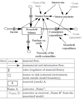
The elaborated dynamic model of the crediting volume system calculates and evaluates household budget balance and budget forming flows. The model includes four basic physical flows (Figure 1). The first flow characterizes income – salary and other income. The second flow describes expenditures – consumption expenditures for food, household maintenance etc., as well as loan and interest payments. The third flow includes an increase in budget balance as a result of the amount of the granted loan credit, and the fourth flow represents the costs associated with the purchase of the loan object.
In order to calculate the household loan burden, the following task must be fulfilled: to determine the time after which the bank will grant a new loan to a household for the purchase of a flat. It is assumed that the bank will grant a loan under the following conditions:
– household pays at least a% of the value of the purchase object; – the sum of loan repayment and interest payments is not less
than b% of household income (loan burden limitation);
– monthly loan repayments are equal during the loan period, and interest payments are calculated from the remainder of the loan;
– loan period is c years;
– interest rate of the loan is d% per year; – the market price of the flat is e LVL;
– household has just received a loan of f LVL under previously mentioned conditions;
– household net income is g LVL per month;
of the loan and loan payments). General flows of the dynamic model for the crediting volumesystem are illustrated in Figure 1.
where: material flow;
nonmaterial and information flow; valve (regulator of material flows);
source or sink (external environment, stock outside model boundary); reservoir (stock) A;
Name A converter „Name”;
[image:4.595.164.441.228.562.2]converter or reservoir „Name B” from the associated model.
Figure 1. Dynamic model of crediting volume system.
In Figure 1, the relations among system dynamic indicators are elaborated. Symbolsillustrating the model and explanatory equations are represented according to generally accepted system dynamics denotations (Sterman, 2000).
INTEGRAL (A, B) – integral from A, but in start time (t0) integral from B;
IF THEN ELSE (A, B, C) – the logical choice operator: if A
condition is simultaneously present(is in force; correct), then an operator gives expression B; otherwise, an operator gives expression C;
A :AND: B – the logical association operator: simultaneous (together) A and B;
DELAY FIXED (A, t, B) delay operator: A – expression whose implementation is delayed for time t, but in the beginning, while expressionAis not used, itoperates expression B.
Model equations:
Household Balance = INTEGRAL (Income + Granted Loan – Consumption Expenditures – Purchase on Credit, 0)
Purchase on Credit = IF THEN ELSE (Necessity of the Credit Commodities >0 :AND: Granted Loan >0, Necessity of the Credit Commodities, 0) (Purchase on credit for the complete sum of necessities is possible if two conditions are present simultaneously: the need to buy on credit exists, and the loan is granted. Otherwise, purchases on credit are not possible.)
Consumption Expenditures = Household Expenditures + Loan Repayment + Interest Payments
Granted Loan = IF THEN ELSE (γ :AND: δ, (Necessity of
the Credit Commodities – Household Budget Balance), 0) (if conditions γ and δ are simultaneously present (are in force, correct), the loan is granted as a difference between necessities and household resources; otherwise, the loan is not granted). where:
γ = Volumeof First Payment * Necessity ofthe Credit Commodities
< Household Budget Balance (verification of whether there are sufficient resources in order to meet the first payment of a% of necessities).
δ = Loan Burden Limitation * Income > (The New Loan / Term of
total loan repayments and interest payments associated with the new and old loan).
The New Loan = Necessity ofthe Credit Commodities – Household
Budget Balance (variables The New Credit, γ and δ are dummy variables; they are not represented in Figure 1, but their application facilitates explanation of the model).
Interest Payments = Loan Volume, * Interest Rate /12
[image:6.595.134.439.379.438.2]In order to ensure operation of the basic flow of granting a loan, two additional flows are needed: one is for loan volume, and the second for loan repayment analysis. These additional flows are represented in Figures 2 and 3.
Figure 2. Model for calculating volume of loan.
The submodel of calculation the loan volumeincludes the following relations among system dynamic indicators:
Loan Repayment = Loan Repayment Volumeper Month
Loan Volume= INTEGRAL (Loan Increase – Loan Repayment,
Initial Loan) (for determining the loan volumeat start time (t0), an Initial Loan indicator is used; then Loan Increase and Loan Repayment are applied to determine the loan volume.)
Loan Increase = Granted Loan
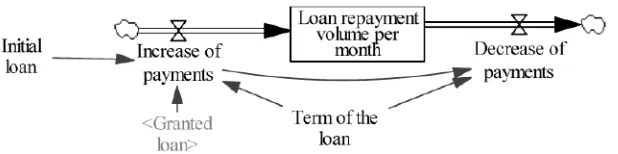
Figure 3. Model for calculating Loan Repayment Volume.
The submodel for calculating Loan Repayment Volumeincludes the following relations among system dynamic indicators:
Loan Repayment Volumeper Month = INTEGRAL (Increase of Payments – Decrease of Payments, 0)
Increase of Payments = (Granted Loan + Initial Loan)/ Term of
the Loan (the indicator Initial Loan differs from zero only in the beginning).
Decrease of Payments = DELAY FIXED (Increase of Payments,
Term of the Loan,0) application of the DELAY FIXED operator
ensures that Loan Repayment Volume(per month) decreases during the term of the loan by the same amount as does the Increase of Payments because of the granted loan.
The elaborated theoretical model is verified in practice by using the following parameters:
First payment a = 0.2 (20%);
Loan burden limitation b = 0.4 (40%);
Term of the loan c = 120 (per month);
Interest rate d = 0.08 (8%);
Necessity of the credit commodities e = LVL 65,000 (till the time when the flat will be purchased);
Initial loan f = LVL 5,000 (only at the beginning);
Household income g = LVL 1,050;
Household expenditures i = LVL 400.
after the purchase of the flat are LVL 425 (40% of the total income). Consequently, all limitations are taken into account.
Analysis of the results indicates that the first actual payment (from household resources) is substantially larger than necessary according to initial conditions (59% against 20%). It means that the first precondition for granting a loan is the capability of a household to cover all costs, including loan repayments and interest payments. For households with a larger difference between income and expenditures, the situation may differ.
This task is quite simple, but it shows that the system dynamic method can be applied in everyday life or in entrepreneurship. But its main advantage is that the model elaborated for entrepreneurship can be applied for forecasting on a macroeconomic level, as is demonstrated further.
2. Modeling of national crediting system
When granting loans to households, financial establishments analyze each particular loan request and from individual loans, the total loan portfolio is formed. Financial establishments make sure that households are capable of paying for loans and thus the overall loan portfolio in the country does not exceed total household solvency. Till now, research on the potential level of the loan burden of households in Latvia has not been conducted despite the fact that this very topical subject is widely discussed among experts. The previously mentioned system dynamic model makes it possible to evaluate the potential level of loan burden in Latvian households. In order to do that, it is necessary to adapt the model to the macro level.
In order to adapt the model to the macro level, first of all, statistical data on the modeling object (including data on population) are necessary. During execution of the project „Elaboration of Latvian entrepreneurial
competitiveness system dynamic forecasting model” (Skribans and Počs,
2008), J. Forrester’smodel for forecasting population size in thesocial economic system (Форрестер, 2003) was adapted to actual conditions
in Latvia. Its results (prognoses of population dynamics) serve as an informative base and data source in this research. Similar use of Forrester’s model in Latvia was made for dynamics of a number of agriculture industry
scientists (Kalniņš et al., 2007).
of children (population under 14 years of age) will decrease. The only population group which will increase in number will be pensioners (population over 65 years of age), which is not favorable to the social economic/social economic system.
According to the data of the Bank of Latvia4, loans by banksto private persons in the summer of 2008 were LVL 6,293.8 mil., which can be set as an initial loan in the new model. According to the data of the Central Statistical Bureau5, income per household member in 2006 year was LVL 259 per month, but expenditures were LVL 209. Unfortunately, more up-to-date information is not available at present; therefore, the data of 2006 are used for the initial loan. During the research, the author realized that old data do not influence the quality of research. Crediting needs are represented as Latvian population’s need for housing (including
flats) (Skribans and Počs, 2008). All other input parameters of the model
(interest rate, term of the loan and others) are constant as in the case of a single household.
Second, it is necessary to change some economic relations in the model. It is not completely correct for multiple population volume with variables of the submodel represented in Figure 3. It will give results only for the period when the necessary sum for the first payment will be accumulated for all solvent households, and all solvent households will acquire dwellings at the same time. Until that period, the potential level of loan burden for households will not be estimated correctly.
In the context of this research, the author concludes the following: if there is an influenceof the first payment on the dwelling acquisition period on the household level, then its influence on the macro level is insignificant. The capability of households to make interest payments and loan repayments in due time is the main factor.
The scheme of the macroeconomic model is not shown in this paper because it is similar to the household model (Figures 1 – 3).
The simulated potential level of the loan burden of Latvian households, estimated by using 2006 year data, was LVL 7,216 mil. in 2006; during the next 10 years it will increase by approximately LVL 29 mil. per month, with constant household income and expenditures. This household crediting level is still not achieved. Analysis of the proportion of household income and expenditures indicates that the potential level of loan burden for Latvian households in 2008 is larger than it was in
2006. Simulated household income, total household expenditures, loan repayments and interest payments from the potential loan are shown in Table 1.
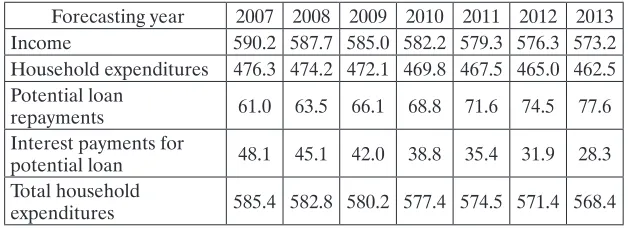
Table 1. Average household potential level of loan burden monthly balance, in LVL.
Forecasting year 2007 2008 2009 2010 2011 2012 2013
Income 590.2 587.7 585.0 582.2 579.3 576.3 573.2
Household expenditures 476.3 474.2 472.1 469.8 467.5 465.0 462.5
Potential loan
repayments 61.0 63.5 66.1 68.8 71.6 74.5 77.6
Interest payments for
potential loan 48.1 45.1 42.0 38.8 35.4 31.9 28.3
Total household
expenditures 585.4 582.8 580.2 577.4 574.5 571.4 568.4
Table 1 shows that during the next five years, income per household will decrease from LVL 590.2 per month to LVL 573.2 per month, or by 2.88%. That is connected to the assumption of constant income and expenditures per person, with the decrease of population, as well as with the fact that some current employees will become pensioners and thus will bring less income to households. Together with the decrease of income, expenditures will also decrease by 2.90% (or from LVL 585.4 per month to LVL 568.4 per month per household). Income will decrease less than expenditures, and thus an increase in welfare is possible.
The aim of the research was not to forecast the increase of income and expenditures but to specify the influence on households of the potential loan that is represented in Table 1. Payments associated with loans (loan repayments and interest payments) can increase, on average, to 15.8% of household expenditures. Taking into account the current income level, this share is rather high, but in comparison with other developed states, it is not that high. For example, the mortgage loan burden for 15% of home owners in the United States is more than a half of their income, and for 38% home owners it is more than 30% of their income.
Conclusions
several important indicators for balancing the household budget: income and expenditures, including those connected with loans. From an analysis of statistics and research data, it may be concluded that in order to achieve the households’ potential level of loan burden in Latvia, it is necessary to increase the loan portfolio by at least 14.7%, which will increase household expenditures by 6.6%.
References
http://en.wikipedia.org/wiki/System_Dynamics (2008). http://www.itl.rtu.lv/mik/?id=1.
Skribans, V., Počs, R. (2008). Latvijas būvniecības nozares attīstības prognozēšanas modelis. Rīga: RTU, 110 pp. In Latvian.
Ieviņa, I., Meļņikova, J., Rozīte K. (2007). “Dinamiskais optimizācijas modelis Latvijas darba tirgus ilgtermiņa līdzsvarošanas prognozēšanai.” LU Raksti. 717. sēj. Vadības zinātne. Rīga: LU Akadēmiskais apgāds. In Latvian.
Sterman, J. (2000). Business Dynamics: Systems Thinking and Modeling for a Complex World. New York: Irwin/McGraw-Hill, 982 pp.
Форрестер, Д. (2003). Мировая динамика. Москва: АСТ, 379 c. In
Russian.
Kalniņš, J.R., Skribans, V., Ozoliņš, G., Bardačenko, V. (2007). Latvijas
lauksaimniecības nozares un zinātnes attīstības stratēģijas izstrādes modelēšanas grupas atskaite. LR Zemkopības ministrija, 48 lpp. In