http://dx.doi.org/10.4236/jmp.2013.412204
Damping-Antidamping Effect on Comets Motion
G. V. López, E. M. Juárez
Departamento de Fsica, Universidad de Guadalajara, Guadalajara, México Email: [email protected]
Received September 12, 2013; revised October 15, 2013; accepted November 11, 2013
Copyright © 2013 G. V. López, E. M. Juárez. This is an open access article distributed under the Creative Commons Attribu- tion License, which permits unrestricted use, distribution, and reproduction in any medium, provided the original work is properly cited.
ABSTRACT
We make an observation about Galilean transformation on a 1-D mass variable system which leads us to the right way to deal with mass variable systems. Then using this observation, we study two-body gravitational problem where the mass of one of the bodies varies and suffers a damping-antidamping effect due to star wind during its motion. For this system, a constant of motion, a Lagrangian and a Hamiltonian are given for the radial motion, and the period of the body is studied using the constant of motion of the system. Our theoretical results are applied to Halley’s Comet.
Keywords: Quantum Computer; Controlled-Not Gate; Diamond
1. Introduction
There is no doubt that mass variable systems have been relevant since the foundation of the classical mechanics and modern physics [1]. These types of systems have been known as Gylden-Meshcherskii problems [2-9], and among these types of systems one could mention: the motion of rockets [10], the kinetic theory of dusty plasma [11], propagation of electromagnetic waves in a disper- sive nonlinear media [12], neutrinos mass oscillations [13] and [14], black holes formation [15], and comets interacting with solar wind [16]. This last system belongs to the so called “gravitational two-body problem” which is one of the most studied and well known system in classical mechanics [17]. In this type of system, one assumes normally that the masses of the bodies are fixed and unchanged during the dynamical motion. However, when one is dealing with comets, besides considering its mass variation due to the interaction with the solar wind, one would like to have an estimation of the the effect of the solar wind pressure on the comet motion. This pressure may produce a dissipative-antidissipative effect on its motion. The dissipation effect must be felt by the comet when this one is approaching to the sun (or star), and the antidissipation effect must be felt by the comet when this one is moving away from the sun. To deal with these types of mass variation problem, it has been pro- posed that the Newton equation must be modified [10] and [18] since the system becomes noninvariant under change of inertial systems (Galileo transformation).
In this paper, we will make a first observation about this statement which indicates that such a proposed mo- dification of Newton’s equation has some problems and rather the use of the original Newton equation is the right approach to dealing with mass variation systems, which was used in previous paper [19] to study two-bodies gravitational problem with mass variation in one of them, where we were interested in the difference of the tra- jectories in the spaces
x v, and
x p,
. As a con-2. Mass Variation Problem and Galileo
Transformation
To simplify our discussion and without losing generality, we will restrict myself to one degree of freedom. Newton equation of motion is given by
d
, , ,
dt m t v F x v t
(1)where m t
v is the quantity of movement, F is thetotal external force acting on the object, m t
andd dt
v x are its time depending mass and velocity of
the body (motion of the mass lost is not considered). Galileo transformations to another inertial frame
Swhich is moving with a constant velocity respect our original frame S are defined as u
x x ut (2) t t (3)
which implies the following relation between the velocity seen in the reference system , , and the velocity seen in the reference system S, Svv,
.
v v u (4)
Multiplying the last term by and making the differentiation with respect to , one gets m t
t
d
, , ,
dt m t v F x v t
(5)where F is given by
, ,
, ,
d
. dm t
F x v t F x ut v u t u
t
(6)
Therefore, Equations (1) and (5) have the same form but the force is different since in addition to the transformed force term F x
ut v , u t,
, one has theterm u m td
dt. This noninvariant form of the forceunder Galilean transformation has lead to propose [10] and [18] that Newton Equation (1) to modify Newton’s equation of motion for mass variation objects, to keep the principle of invariance of equation under Galilean transformations, of the form
d
, ,
d
, dm t v
m t F x v t w
t dt (7)
where is the relative velocity of the escaping mass with respect the center of mass of the object. When one does a Galilean transformation on this equation, one gets
w
d
, , , dv
m t F x v t
t
where F is given by
, ,
, ,
d
, dm t
F x v t F x ut v u t w
t
(9)
which has the same form as Equation (7). However, assume for the moment that wconstant and F0.
So, from Equation (7), it follows that
0
0
ln ,
w
m t
v t v
m
(10)
where m0 m
0 . In this way, if we have a massvariation of the for
0e tm t m (for example), one
would have a velocity behavior like
0 ,v t v w t (11)
which is not acceptable since one can have v> 0,
0
v and v< 0 depending on the value w t . Even
more, since for F 0, the equation resulting in the
reference system S is the same, i.e. in S one gets
the same type of solution,
0
0
ln m t
v t v
m
(12)
which is independent on the relative motion of the reference frames, and this must not be possible due to relation (4).
In addition, it worths to mention that special theory of relativity can be seen as the motion of mass variation problem, where the mass depends on the velocity of the particle of the form
2
1 20 1 2
m v m v c , with c
being the speed of light. This system is obviously not invariant under Galilean transformation, and given the force, Newton’s equation motion is always kept in the same form to solve a relativistic problem,
d m v v dtF x v t, , , [20] and [1].
3. Mass Variation and Equations of Motion
Having explained and clarify the problem of mass va- riation [21], Newton’s equations of motion for two bodies interacting gravitationally, seen from arbitrary inertial reference system, and with radial dissipative- antidissipative force acting in one of them are given by
1 1 2
1 3 1
1 2
d d
d d
Gm m m
t t
r
r r
r r 2
(13)
(8)
and
1 2 2
2 1 2
2 3 2 1
1 2
2 1
d d
d
,
d d d
r Gm m
m
t t t
r r
r r r r
r r
r r 2 1
(14)where and 2 are the masses of the two bodies,
1 1
1
m
1 1, ,
m
x y z
r and r2
x y z2, ,2 2
6.67 10G
are their vectors positions from the reference system, is the gravitational constant
11m /3 Kg sG 2
, is the nonnegative constant parameter of the dissipative- antidissipative force, and
2
2
1 2 2 1 2 1 2 1 2 1
2
x x y y z z
r r r r is
the Euclidean distance between the two bodies. Note that if > 0 and d r1r2 dt> 0 one has dissipation since
the force acts against the motion of the body, and for
1 2
dr r dt0 one has anti-dissipation since the force
pushes the body. If < 0 this scheme is reversed and corresponds to our actual situation with the comet mass lost.
It will be assumed the mass 1 of the first body is
constant and that the mass 2 of the second body
varies. Now, It is clear that the usual relative, , and center of mass, , coordinates defined as 2 1
m m
r
R r r r
and
1 1r m2r
r
2 1 2 are not so good to
describe the dynamics of this system. However, one can consider the case for 1 2 (which is the case star-comet), and consider to put our reference system just on the first body 1
. In this case, Equation (13) and Equation (14) are reduced to the equatioR m m
n m m 0 m
2 2 1 22 2 3 2
d d ˆ,
d d
Gm m r
m m
t t r
r r r r (15)
where one has made the definition rr2
x y z, ,
, ris its magnitude, 2 2 2
r x y z and ˆrr r is the
unitary radial vector. Using spherical coordinates
r, ,
,sin cos , sin sin , cos ,
xr yr zr (16)
one obtains the following coupled equations
2 2 2
1 22 sin 2 2
Gm m
m r r r m r r
r
2
(17)
22 2 sin cos
m rrr
m r2 ,. (18) and
2 2 sin sin 2 cos 2 sin
m r r r m r (19)
Taking 0 as solution of this last equation, the resulting equations are
2
1 22 2 2 ,
Gm m
m r r m r r
r
2
(20) and
2 2 2 0
m rr m r . (21)
From this last expression, one gets the following con- stant of motion (usual angular momentum of the system)
2
2 ,
l m r (22)
and with this constant of motion substituted in Equation (20), one obtains the following one-dimensional equation of motion for the radial part
2 2
2
1 2
2 2 2
2 2 2
d d .
d d l Gm m r r r
m t m
t r m r
3 (23)
Now, let us assume that 2 is a function of the
distance between the first and the second body,
m
2 2
m m r . Therefore, it follows that
2 2 ,
m m r (24)
where m2 is defined as m2 dm2 dr. Thus, Equation
(23) is written as
2 2
2
1 2
2 2 2 3
2 2 d d , d d l Gm m r r m t
t r m r
(25)
which, in turns, can be written as the following autono- mous dynamical system
2
2
1 2
2 2 3
2 2 d d ; . d d l Gm m r v v v
t t r m r m
(26)
Note from this equation that 2 is always a non-
positive function of since it represents the mass lost rate. On the other hand,
m r
is a negative parameter in our case.
4. Constant of Motion, Lagrangian and
Hamiltonian
A constant of motion for the dynamical system (26) is a function KK r v
, which satisfies the partial dif-ferential equation [22]
2
2
1 2
2 2 3
2 2 0. l Gm m K K v v
r r m r m
v
(27)
The general solution of this equation is given by [23]
,
,
,K x v F c r v (28)
where F is an arbitrary function of the characteristic
curve c r
,v which has the following expression
2 2 2 2 2 2 2 1 22 2 3
2 , e 2 2 e d r r
c r v m r v
l Gm
m r r
r m r
, (29)and the function
r has been defined as
2 d . r r m r
(30) During a cycle of oscillation, the function m2
r canbe different for the comet approaching the sun and for the comet moving away from the sun. Let us denote
2
m r for the first case and for the second
case. Therefore, one has two cases to consider in Equa- 2
tion (28) which will denoted by
. Now, if 2om
denotes the mass at aphelium (+) or perielium (−) of the comet,
2 2oF c c m represents the functionality in
Equation (28) such that for m2 constant and equal
zero, this constant of motion is the usual gravitational energy. Thus, the constant of motion can be chosen as
, 2 2o
K c r v m, that is,
2 2 2 2 e , 2 r eff om r 2
K v V r
m eff V (31) where the effective potential has been defined as
1 22
2 2 2 2 2
e d
eff o o
m r r l
Gm r
V r
m r m r
e2 d
3rr
(32) This effective potential has an extreme at the point
defined by the relation r*
2 2
* 2 r* 1
l r m
Gm
(33) which is independent on the parameter and depends on the behavior of m2
r . This extreme point is aminimum of the effective potential since one has
2 2 eff V r * d 0. d
r r
(34) Using the known expression [24-26] for the Lagran- gian in terms of the constant of motion,
2, d
, K r v v,
L r v
v
v
(35)the Lagrangian, generalized linear momentum and the Hamiltonian are given by
r 2
2 2 2 2 e ,2 o eff
m r
L v V
m
r (36)
2 2 2 2 o m r
e r ,v p
m
(37) and
e . 2 2 2m p2 2
2 o
r eff
H V
r m r (38) The trajectories in the space
x v, are determined bythe constant of motion (31). Given the initial condition , the constant of motion has the specific value
r vo, o
e
, o 2 2 2 2 2 o r oo o eff o
m r 2
K v V
m
r
(39)
and the trajectory in the space
r v, is given by
1 2 e . 2 2 2 2 o o eff mv K V r
m r
r (40)
Note that one needs to specify o also to determine
Equation (22). In addition, one normally wants to know the trajectory in the real space, that is, the acknowledg- ment of rr
. Since one has that
d d
v r t d dr and Equations (22) and (40), it
follows that
2 2 2 2 e d . 2 o r ro o r
o eff
m r r
l r
m r K V r
(41)The half-time period (going from aphelion to peri- helion (+), or backward (−)) can be deduced from Equa- tion (40) as
2 1 2 1 2 2 e d 1 , 2 r r r o o effm r r
T
m K V r
(42)where 1 and 2 are the two return points resulting
from the solution of the following equation
r r
, 1, 2.eff i o
V r K i (43)
On the other hand, the trajectory in the space
r p,
is determine by the Hamiltonian (38), and given the same initial conditions, the initial po and Ho are obtainedfrom Equations (38) and (37). Thus, this trajectory is given by
2 1 2 2 2 2e r .
o eff o
m r
p H V
m
r
(44) It is clear just by looking the expressions (40) and (44) that the trajectories in the spaces
r v, and
r p,
must be different due to complicated relation (37) be- tween and [19]. v p
5. Mass-Variable Model and Results
As a possible application, consider that a comet looses material as a result of the interaction with star wind in the following way (for one cycle of oscillation)
2 1
2 2 1
2
2 2 1
1 e , < 0 1 e i , > 0
r i
r r i
m r v
m r
m r b v
(45)
where the parameters b> 0 and > 0 can be chosen to math the mass loss rate in the incoming and outgoing cases. The index “i” represent the ith-semi-cycle, being
2i1
r and r2 1i the aphelion
ra
and perihelion
rppoints ( is given by the initial conditions, and one has that o
r
o 2
m r mo). For this case, the functions
rand
r are given by
1 ln e
r 1 ,a r m
and
1
ln
1 e r rp
.p p
r r m b
b m
(47)
2
2 2
e
2 1 2 2
e 1 e 1 e
2 a
r
r m r r
a a a
m m m
,
(48) where we have defined ma m2
ra and mp m2
rp .Using the Taylor expansion, one gets and
2
2 2
2 2
e 2 e 1 2 2 e
e 1 1
2
p p p
p
r
b m r r r r
r
p
p p p
m b p
p
m b
m b m b m b m b
m b
.
(49)
The effective potential for the incoming comet can be written as
1 2 2
1 2
1 e ,
2
a
r m a
eff
a
Gm m l
V r W r
r m r
, ,
(50)and for the outgoing comet as
2 1
2
2
2 2
1 2
e
, , ,
p
p
a eff
a r m b
m b p
Gm m l
V r
r m r
W r
m b
(51)
where 1 and W2 are given in the Appendix. We will
use the data corresponding to the sun mass
and the Halley comet [27] and [28]
W
1.9891 1 0 Kg30
14
2.3 10 Kg, 0.6 au,
c p
m r
29 2
35 au, 10.83 10 Kg m /s, a
r l
11
(52) with a mass lost of about per cycle of oscillation. Although, the behavior of Halley comet seem to be chaotic [29], but we will neglect this fine detail here. Now, the parameters
2.8 10 Kg
m
and " appearing on the mass lost model, Equation (45), are determined by the chosen mass lost of the comet during the approaching to the sun and during the moving away from the sun (we have assumed the same mass lost in each half of the cycle of oscillation of the comet around the sun). Using Equation (50) and Equation (51) in the expression (40), the trajectories can be calculated in the spaces (
"
b
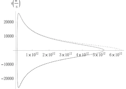
[image:5.595.54.333.65.411.2] [image:5.595.63.542.80.230.2]v r, ).
Figure 1 shows these trajectories using
10
2 10 Kg
m
( o r m m0.0087% ) f o r 0
and (continuos line), and for 3 Kg/m (dashed line), starting both cases from the same aphelion distance. As one can see on the minimum, dissipation causes to reduce a little bit the velocity of the comet, and the antidissipation increases the comet velocity, reaching a further away aphelion point. Also, when only mass lost is considered the comet returns to aphelion point
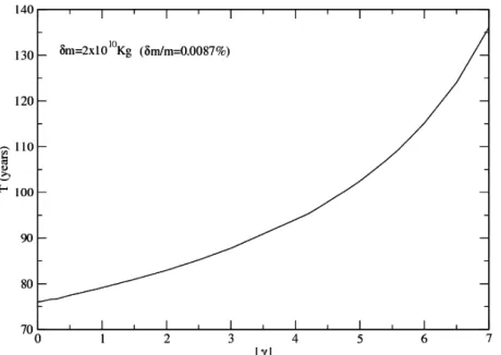
a little further away from the initial one during the cycle of oscillation. Something related with this effect is the change of period as a function of mass lost
0
0
. This can be see on Figure 2, where the period is calculatedstarting always from the same aphelion point
ra11Kg . Note
that with a mass lost of the order (Halley comet), which correspond to
2.8 10 12%
m m
, the comet is well within 75 years period. The variation of the ratio of the change of aphelion distance as a function of mass lost
0
is shown on Figure 3. On Figure 4, the masslost rate is kept fixed to m m0.0087%, and the
variation of the period of the comet is calculated as a function of the dissipative-antidissipative parameter
< 0
(using for convenience). As one can see, antidissipation always wins to dissipation, bringing about the increasing of the period as a function of this parameter. The reason seems to be that the antidissi- pation acts on the comet when this ones is lighter than when dissipation was acting (dissipation acts when the comet approaches to the sun, meanwhile antidissipation acts when the comet goes away from the sun). Since the period of Halley comets has not changed much during many turns, we can assume that the parameter must vary in the interval
0.01, 0 Kg/
m. Finally, Figure 5
r v, [image:5.595.57.287.264.416.2] [image:5.595.316.533.546.699.2]Figure 2. Period of the comet as a function of the mass lost ratio.
Figure 3. Ratio of aphelion distance change as a function of the mass lost rate.
Figure 4. Period of the comet as a function of the parameter .
[image:6.595.60.288.287.452.2]shows the variation, during a cycle of oscillation, of the ratio of the new aphelion
ra to old aphelion
ra asFigure 5. Ratio of the aphelion increasing as a function of the parameter .
6. Conclusion and Comments
odified Newton as some problems. We have shown that the proposed m
equation for mass variation systems h
Therefore, we have considered that it is better to keep Newton’s equations of motion for mass variable systems to have a consistent approach to these problems. Having this in mind, the Lagrangian, Hamiltonian and a constant of motion of the gravitational attraction of two bodies were given when one of the bodies has variable mass and the dissipative antidissipative effect of the solar wind is considered. By choosing the reference system in the massive body, the system of equations is to reduce 1-D problem. Then, the constant of motion, Lagrangian and Hamiltonian were obtained consistently. A model for comet-mass-variation was given, and with this model, a study was made of the variation of the period of one cycle of oscillation of the comet when there are mass variation and dissipation-antidissipation. When mass va- riation is only considered, the comet trajectory is moving away from the sun, the mass lost is reduced as the comet is farther away (according to our model), and the period of oscillations becomes bigger. When dissipation anti- dissipation is added, this former effect becomes higher as the parameter becomes higher.
REFERENCES
[1] G. López, L. A . Hernández and J. C. Salazar, International Journal of Theoretical Physics,
.org/10.1002/asna.18841090102 . Barrera, Y. Garibo, H
Vol. 43, 2004, p. 1.
[2] H. Gylden, Astronomische Nachrichten, Vol. 109, 1884, pp. 1-6. http://dx.doi
[3] I. V. Meshcherskii, Astronomische Nachrichten, Vol. 132, 1893, p. 93.
[4] I. V. Meshcherskii, Astronomische Nachrichten, Vol. 159, 1902, p. 229.
[image:6.595.60.290.493.656.2]ttp://dx.doi.org/10.1002/asna.19021582202 [5] E. O. Lovett, Astronomische Nachrichten, Vol. 158, 1902,
pp. 337-344. h
[6] J. H. Jeans, MNRAS, Vol. 85, 1924, p. 2.
[7] L. M. Berkovich, Celestial Mechanics, Vol. 24, 1981, pp. 407-429. http://dx.doi.org/10.1007/BF01230399
physics
.
ol. 84, 2000, pp. 3594-3597. [8] A. A. Bekov, Astron. Zh., Vol. 66, 1989, p. 135.
[9] C. Prieto and J. A. Docobo, Astronomy & Astro , Vol. 318, 1997, p. 657.
[10] A. Sommerfeld, “Lectures on Theoretical Physics,” Vol. 1, Academic Press, 1964
[11] A. G. Zagorodny, P. P. J. M. Schram and S. A. Trigger, Physical Review Letters, V
http://dx.doi.org/10.1103/PhysRevLett.84.3594
[12] O. T. Serimaa, J. Javanainen and S. Varró, Physical Re-view A, Vol. 33, 1986, pp. 2913-2927.
http://dx.doi.org/10.1103/PhysRevA.33.2913 [13] H. A. Bethe, Physical Review Letters,
1305-1308. Vol. 56, 1986, pp. http://dx.doi.org/10.1103/PhysRevLett.56.1305
[14] E. D. Comm
tions of Leptons and Quarks,” Cambridge Uins and P. H. Bucksbaum, “Weak Interac-niv
Springer-Verlag, 1998. ersity Press, Cambridge, 1983.
[15] F. W. Helhl, C. Kiefer and R. J. K. Metzler, “Black Holes: Theory and Observation,”
http://dx.doi.org/10.1007/b13593
[16] P. W. Daly, Astronomy & Astrophysics, Vol. 226, 1 318.
989, p. [17] H. Goldstein, “Classical Mechanics,” Addison-Wesley,
1950.
[18] A. R. Plastino and J. C. Muzzio, Celestial Mechanics and Dynamical Astronomy, Vol. 53, 1992, pp. 227-232. http://dx.doi.org/10.1007/BF00052611
[19] G. López, International Journal of Theoretical Physics, 773-006-9085-4
Vol. 46, 2007, pp. 806-816. http://dx.doi.org/10.1007/s10
niversity athematicians, Mechanics I,” al Equations of First Order [20] C. Møller, “Theory of Relativity,” Oxford U
Press, Oxford, 1952. [21] M. Spivak, “Physics for M
Publish or Perish Inc., 2010. [22] G. López, “Partial Differenti
and Their Applications to Physics,” World Scientific, 1999. http://dx.doi.org/10.1142/4006
[23] F. John, “Partial Differential Equations,” Springer-Verlag, ta Phys. Austr., Vol. 51, 1979, p. 193. New York, 1974.
[24] J. A. Kobussen, Ac
[25] C. Leubner, Physics Letters A, Vol. 86, 1981, pp. 68-70. http://dx.doi.org/10.1016/0375-9601(81)90166-3
[26] G. López, Annals of Physics, Vol. 251, 1996, pp. 372-383. http://dx.doi.org/10.1006/aphy.1996.0118
[27] G. Cevolani, G. Bortolotti and A. Hajduk, Il Nuovo Ci- mento C, Vol. 10, 1987, pp. 587-591.
http://dx.doi.org/10.1007/BF02507255
[28] J. L. Brandy, Journal of the British Astronomical Asso- echeslavov, Astronomy & ciation, Vol. 92, 1982, p. 209.
Appendix
r W1 and W2:
Expression fo
4 2 2 1 2 2 3 2 2 2 2 1 2 2 2 1 e2 1 4
2
1 1
4 e 3 1 3
2
3 e 2
2 2 e 1 1
2 1 e e 2 2 p r i i o p r i i p r p r i i
p r p r
p p Gm
W pE pr p p E p r
r m
p p p p
E p r p rE p r
r
p p p
p E p r p rE p r
r r p p l p p m r
2 22 1 2 1 2 2 2
2
2 2
2 2
2 2 2 3 2 2
1
1 e e
2 1
e e e
2
2 1
2 1
2
2 1 1
p r p r
p r p r p r
i
i i
i i
p p p
p p r
p r p r p r E p r
p p p r
E p r p r E p r
p r E p r p r E p r
(A1)
where ma is the mass of the body at the aphelion, and we have made the definitions
2 . a p m
(A2)
2 2 2 2 2 2 2 3 2 32 2 2
2
1
e 2
1 e e
2
1 e
e 3 3
e e 3 3 2 2
1 e 1 e
2 2
q r
q r q r
o p p q r q r i i p q r q r i i p
q r q r
i i
p
q q
Gm q
W
r m q
m m q
q q
q E q r q rE q r
m q r
q
q rE q r E q r
m q r
q q q q
qE q r E q r
m q
2 2 1 1 3 2 2 2 2 2 2 2 22 2 2
2 2
4 e 2 e
2 2
2 e
e 1 1 e 1 1
1 e e
2 2
1 2 2 e
i p
q r q r
i i
p p
q r
q r q r
i i p q r q r i q p p
E q r
m q
q
E q r E q r
m q m q r
q
q rE q r q rE q r
r m q r
q q
l q
q E q r
r
m m q m q r
r q r q r
2 2 12 2 2 1 2
2
e 1 1 e 1
q r i q r q r i p
E q r
q
r q r q r E q r
m q r
where mp is the mass of the body at the perihelion, and we have made the definition
2p
q
m b
(A4)
and the function Ei is the exponential integral,
e d ti z
E z t
t