
http://dx.doi.org/10.4236/jmf.2016.62028
How to cite this paper: Fadugba, S.E. and Nwozo, C.R. (2016) Valuation of European Call Options via the Fast Fourier Trans- form and the Improved Mellin Transform. Journal of Mathematical Finance, 6, 338-359.
http://dx.doi.org/10.4236/jmf.2016.62028
Valuation of European Call Options via the
Fast Fourier Transform and the
Improved Mellin Transform
Sunday Emmanuel Fadugba1, Chuma Raphael Nwozo2*
1Department of Mathematical Sciences, Ekiti State University, Ado Ekiti, Nigeria 2Department of Mathematics, University of Ibadan, Ibadan, Nigeria
Received 28 March 2016; accepted 28 May 2016; published 31 May 2016
Copyright © 2016 by authors and Scientific Research Publishing Inc.
This work is licensed under the Creative Commons Attribution International License (CC BY).
http://creativecommons.org/licenses/by/4.0/
Abstract
This paper considers the valuation of European call options via the fast Fourier transform and the improved Mellin transform. The Fourier valuation techniques and Fourier inversion methods for density calculations add a versatile tool to the set of advanced techniques for pricing and man-agement of financial derivatives. The Fast Fourier transform is a numerical approach for pricing options which utilizes the characteristic function of the underlying instrument’s price process. The Mellin transform has the ability to reduce complicated functions by realization of its many properties. Mellin’s transformation is closely related to an extended form of other popular trans-forms, particularly the Laplace transform and the Fourier transform. We consider the fast Fourier transform for the valuation of European call options. We also extend a framework based on the Mellin transforms and show how to modify the method to value European call options. We obtain a new integral equation to determine the price of European call by means of the improved Mellin transform. We show that our integral equation for the price of the European call option reduces to the Black-Scholes-Merton formula. The numerical results show that the tremendous speed of the fast Fourier transform allows option prices for a huge number of strikes to be evaluated very ra-pidly but the damping factor or the integrability parameter must be carefully chosen since it con-trols the intensity of the fluctuations and the magnitude of the functional values. The improved Mellin transform is more accurate than the fast Fourier transform, converges faster to the Black- Scholes-Merton model, provides accurate comparable prices and the approach can be regarded as a good alternative to existing methods for the valuation of European call option on a dividend paying stock.
Keywords
Black-Scholes Partial Differential Equation, European Call Option, Fast Fourier Transform,
Improved Mellin Transform, Mellin Transform
1. Introduction
In the past decades, option pricing has become one of the major areas in modern financial theory and practice. Since the introduction of the celebrated Black-Scholes option-pricing model, which assumes that the underlying stock price follows a geometric Brownian motion (GBM), there is an explosive growth in trading activities on derivatives in the worldwide financial markets [1]. [2] developed a fast Fourier method to compute option prices for a whole range of strikes. This method makes use of the characteristic function of the underlying asset price. The use of the fast Fourier transform method is motivated by the following reasons: the algorithm has speed ad-vantage. This enables the Fourier transform algorithm to calculate prices accurately for a whole range of strikes. The characteristic function of the log-price is known and has a simple form for many models considered in lite-rature while the density is often not known in the closed form. Option values can be calculated numerically by multiplying a payoff function with transition density of an underlying asset, then taking its discounted expecta-tion with respect to an equivalent martingale measure (see [3] and [4]). This method of martingale pricing is of-ten computed with respect to the space of the asset, despite ofof-ten posing more challenging. In 2002, [5] pio-neered the method of using the Mellin transform to solve the associated Black-Scholes partial differential equa-tion for a European call opequa-tion. Mellin transforms in opequa-tion theory were also introduced by [6]. They derived integral representations for the price of European and American basket put options using Mellin transform tech-niques. [7] derived integral representations for the prices of European and American put options on a basket of two-dividend paying stocks using integral method based on the double Mellin transform. They showed that by the decomposition of the integral equation for the price of American basket put option, the integral equation for the price of European basket put option can be obtained directly. The Mellin transform method for the valuation of the American power put option with non-dividend and dividend yields respectively was considered by [8]. They used the Mellin transform method to derive the integral representations for the price and the free boundary of the American power put option. They also extended their results to derive the free boundary and the funda-mental analytic valuation formula for perpetual American power put option. For mathematical backgrounds, sporadic applications of transform methods in financial contexts see [9]-[18] just to mention a few.
In this paper, we consider the valuation of the European call option via the fast Fourier transform and the im-proved Mellin transform on a dividend paying stock. The rest of the paper is organized as follows. Section 2 presents overview of the Black-Scholes-Merton model. Section 3 considers some fundamental properties of the Fourier transform and the fast Fourier transform method for the valuation of European options. In Section 4, we present the Mellin transform, some basic properties and the application of the improved Mellin transform in the theory of European call option valuation. Section 5 presents some numerical examples and discussion of results. Section 6 concludes the paper.
2. Black-Scholes-Merton-Like Valuation Formula
We consider a market where the underlying asset price St, 0≤ ≤t T is governed by the stochastic differential equation of the form
(
)
dSt = r−q S ttd +σS Wtd t, 0<St < ∞ (1)
where σ is the volatility, r is the riskless interest rate, q is the dividend yield and Wt is a one-dimensional
Wiener process. Standard arbitrage arguments show that any derivative u S t
(
t,)
written on St must satisfythe partial differential equation [19].
Theorem 1 [15]: Let n t
S denote the price of the underlying asset, σ >0 the volatility, r the riskless inter-est rate, n the power of the option, q the dividend yield and Wt the Wiener process. If the underlying price of
the asset n t
S follows a random process (Geometric Wiener process) in
(
)
1(
)
2d 1 d d
2 σ σ
= − + − +
n n n
t t t t
Then the explicit formula for the evolution of the underlying price of the asset is given by
2 0
1 exp
2σ σ
= − − +
n n
T T
S S n r q T n W (3) Proof: Let
( )
, ln= n = n
t t
u u S t S (4) Differentiating (4) we have
( )
( )
( )
( )
( )
2
2 2
, 1 , 1 ,
, , 0
∂ ∂ ∂
= = − =
∂
∂ ∂
n n n
t t t
n n n n
t t
t t
u S t u S t u S t
t
S S S S (5)
Recall from Ito’s lemma and using (2) for any derivative u S t
( )
tn, we have( )
( )
( )
( )
( )
( )
2 2
2
, , , ,
d , d d
2
∂ ∂ ∂ ∂
= + + +
∂ ∂ ∂
∂
n n n n
t t t t
n
t n n n t
t t t
u S t u S t g u S t u S t
u S t f t g W
t S S S (6)
From (2), we can write for
(
)
1 2( 1) ,
2 σ σ
= − + − =
n n
t t
f n r q n n S g n S (7) Substituting (4), (5) and (7) into (6) and rearranging the terms, we have
(
)
(
)
(
)
( )
( )
2
2 2 2
2
1 1
d ln 1 d
2
1 1 1
d d
2
σ
σ σ
= − + −
−
+ +
n n
t t n
t
n n
t t n t
n
t t
S n r q n n S t
S
n S t n S W
S S
(8)
Therefore,
(
)
(
)
1 2d ln d d
2 σ σ
= − − +
n
t t
S n r q n t n W (9) Thus, lnStn is a Brownian motion with drift parameter
2
1 2 σ
−
nr n and variance parameter nσ
2
. To
de-rive an explicit formula for the evolution of the stock price, we integrate (9) from 0 to T to obtain
2 0
1 ln
2σ σ
= − − +
n T
T n
S
n r q T n W
S (10)
2 0
1 exp
2σ σ
= − − +
n n
T T
S S n r q T n W (11) Equation (11) can also be written as
2 0
1 exp
2σ σ
= − − +
n n
T
S S n r q T n Z T (12) where Z∼N(0,1). Therefore the stock dynamic follows a log-normal distribution. For n = 1, (12) becomes
2 0
1 exp
2σ σ
= − +
T
Theorem 2: Let the underlying asset price n t
S follows a lognormal random walk (geometric Wiener process)
(
)
1(
)
2d 1 d d
2 σ σ
= − + − +
n n n
t t t t
S n r q n n S t n S W
using the Ito’s lemma, under the standard arbitrage argument the Black-Scholes partial differential equation for any derivative
( )
n,t
u S t on n t
S for vanilla power option which pays dividend yield is given by
( )
(
) (
)
( ) ( ) ( )
( )
( )
2 2 2
2
, 1 , 1 ,
1 ,
2σ 2 σ
∂ ∂ ∂
+ − + − + =
∂ ∂ ∂
n n n
t n t n t n
t n t n t
t
t
u S t u S t u S t
n n r q S nS ru S t
t S S (14)
Remark 1
1) For n = 1, (14) is known as the regular Black-Scholes-Merton partial differential equation which is given by
(
) ( )
(
)
2(
)
(
)
2 2 2
, , 1 ,
, 2σ
∂ ∂ ∂
+ − + =
∂ ∂ ∂
t t t
t t t
t t
u S t u S t u S t
r q S S ru S t
t S S (15)
2) If u S t
( )
t, =u S tc( )
t, is a vanilla call option, then (15) becomes the Black-Scholes-Merton partial differen-tial equation for a vanilla call option given by(
) ( )
(
)
2(
)
(
)
2 2 2
, , 1 ,
, 2σ
∂ ∂ ∂
+ − + =
∂ ∂ ∂
c t c t c t
t t c t
t t
u S t u S t u S t
r q S S ru S t
t S S (16)
3) The solution to (16) is obtained as
(
)
( )
( )( )
( )1 2
, = e−q T t− − e−r T t−
c t t
u S t S N d KN d (17) where
(
)
(
)
(
)
(
)
(
)
2 2
1 2 1
ln ln
2 2
,
σ σ
σ
σ σ
+ − + − + − − −
= = = − −
− −
t t
S S
r q T t r q T t
K K
d d d T t
T t T t
and N
( )
. is the commutative distribution function for the standard normal distributionEuropean Options
Definition 1
European is an option that can be exercised only at the expiry date with linear payoff. European option comes in two forms namely European call and put options.
Definition 2
A European call option is an option that can be exercised only at expiry and has a linear payoff given by the difference between underlying asset price at maturity and the exercise price.
Definition 3
A European put option is an option that can be exercised only at expiry and has a linear payoff given by the difference between the exercise price and underlying asset price at maturity.
For a European option on the underlying price of the asset St with exercise price K and time to expiry T, we
have the payoff for the European call option as
(
,) (
= −)
+c T T
E S T S K 18) The payoff for the European power put option is given as
(
,) (
= −)
+p T T
E S T K S (19) Setting uc
(
S tt,)
=Ec(
S tt,)
in (15), then we have the Black-Scholes-Merton partial differential equation for(
) ( )
(
)
2(
)
(
)
2 2 2
, , 1 ,
, 2σ
∂ ∂ ∂
+ − + =
∂ ∂ ∂
c t c t c t
t t c t
t t
E S t E S t E S t
r q S S rE S t
t S S (20)
with boundary conditions
(
,)
→ ∞ as → ∞ on 0,[
)
c t t
E S t S T (21)
(
,)
→0 as →0 on 0,[
)
c t t
E S t S T (22)
and final time condition given by
(
,) (
= −)
+=( )
on 0,[
∞)
c T T T
E S T S K g S (23)
3. Fast Fourier Transform Method for the Valuation of European Call Options
This section presents some fundamental properties of Fourier transform and the fast Fourier transform method for the valuation of European options. The fast Fourier transform was first proposed by [2]. It ensures that the Fourier transform of the call price exist by the inclusion of a damping factor. Moreover, Fourier inversion can be accomplished by the fast Fourier transform in this case. The tremendous speed of the fast Fourier transform al-lows option prices for a huge number of strikes to be evaluated very rapidly.3.1. Fourier Transforms
Definition 4
Suppose f x
( )
is absolutely integrable in(
−∞ ∞,)
, i.e.( )
d∞
−∞
< ∞
∫
f x x , then the Fourier transform of( )
f x is defined as
( )
(
)
( )
( )
( )
e d∞
−∞
= =
∫
ikxF f x k f k f x x (24) The Fourier transform is a generalization of the complex Fourier series.
Definition 5
If f x
( )
is square integrable, then the inverse Fourier transform of f k( )
is defined as( )
(
)
( )
( )
1 1
e d 2π
ikx
F f k f x f k k
∞
− −
−∞
= =
∫
(25)
3.2. Some Fundamental Properties of Fourier Transforms
Let the Fourier transform of f x
( )
be defined as F f x(
( )
)
( )
k = f k( )
then the following fundamental prop-erties hold as follows:1) Scaling Property
( )
(
)
( )
1e dikx k
F f υx f υx x f
υ υ
∞
−∞
= =
∫
(26)2) Shifting/Translation Property
(
)
(
)
( )
(
)
( )
( )( )
( )
0
0 0
0 0 e d e d
e e d e
ik z x ikx
ikx ikz ikx
F f x x k f x x x f z z
f z z f k
∞ ∞
+
−∞ −∞
∞
−∞
− = − =
= =
∫
∫
∫
(27)( ) ( )
( ) ( )
( )
de d d
∞
−∞
= =
∫
ikx
F f x k ik f x x ikf k
x (28)
This process can be iterated for the nth derivative to yield
( ) ( )
( ) ( )
( ) ( )
d
e d d
∞
−∞
= =
∫
n
n ikx n
n
F f x k ik f x x ik f k
x (29)
Thus, a differentiation converts to multiplication in Fourier space.
4) Convolution Property
( ) ( )
(
)
( )
( ) (
)
( )
(
)
(
( )(
)
)
( )
(
)
(
( )(
)
)
( ) ( )
e d d
e d e d
e d e d
∞ ∞
−∞ −∞ ∞ ∞
′ − ′
−∞ −∞
∞ ∞
′ − ′
−∞ −∞
′ ′ ′
∗ = −
′ ′ ′
= −
′ ′ ′
= −
=
∫ ∫
∫ ∫
∫
∫
ikx
ik x x ikx
ik x x ikx
F f x g x k f x g x x x x
f x x g x x x
f x x g x x x
f k g k
(30)
where
( ) ( )
( ) (
)
df x g x f x g x x x
∞
−∞
′ ′ ′
∗ =
∫
− (31)5) Linear Property
( )
( )
(
)
( )
(
( )
( )
)
( )
( )
( )
( )
1 2 1 2
1 2
1 2
e d
e d e d
kix
kix kix
F a f x a g x k a f x a g x x
a f x x a g x x
a f k a f k ∞
−∞
∞ ∞
−∞ −∞
+ = +
= +
= +
∫
∫
∫
(32)
3.3. The Fast Fourier Transforms
The fast Fourier transform (FFT) is proposed by [20]. The fast Fourier transform is an efficient algorithm for computing the discrete Fourier transform of the form;
( )
1
2π
exp , 1, 2, 3, ,
ρ ρ ρ
=
−
= =
∑
N j j
i
m j x N
N (33)
where N is typically a power of two. Equation (33) reduces the number of multiplications in the required N
summations from an order of N2 to that of
(
Nlog2N)
, a very considerable reduction. Let p and j be writtenas binary numbers i.e. ρ=2ρ1+ρ0 and j=2j1+ j0 with j1,j0,ρ ρ1, 0∈
{ }
0,1 , then (33) becomes(
)
(
)(
)
( )( )( )
( ) ( ) ( )
1 0
0 1
1 0 1 0 0 1 0 1 0
1 0 1 0
0 1 0 1
1 1
1 0 1 0 1 0 ,
0 0
1 1 1 1
2 2 2 2
, ,
0 0 0 0
2π
, exp 2 2
ρ ρ ρ ρ
ρ ρ ρ ρ
= =
+ + +
= = = =
−
= + +
= =
∑ ∑
∑ ∑
∑ ∑
j j
j j
j j j j p
j j j j
j j j j
i
m j j x
N
A x A A x
(34)
The fast Fourier transform can be described by the following three steps as
(
)
( )(
)
(
)
( )(
)
(
)
01 0 1 0
0 1
1 1
1 1
2 2
1 2 1
0 0 , 0 0 0 0
0 0
2
0 1 0 1
, , , , ,
, ,
ρ ρ ρ
ρ ρ ρ
ρ ρ
+
= =
= =
=
∑
j∑
jj j
j j
m j x A m j m j A
m p p m
(35)
[20] showed that it was in fact possible to have the discrete Fourier transform evaluated with O N
(
log2N)
arithmetic operations. This O N
(
log2N)
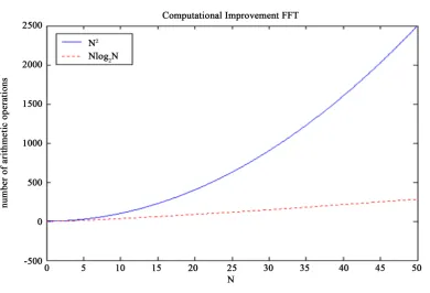
algorithm is called the fast Fourier transform. As a matter of fact, ef-ficient methods for evaluating the discrete Fourier transform have already been devised as long ago as in 1805 by Gauss. However, the world was dormant until 1965. Figure 1 illustrates the huge differences between
( )
2O N and O N
(
log2N)
.The basic idea of the fast Fourier transform is to develop an analytic expression for the Fourier transform of the option price and to get the price by means of Fourier inversion.
By means of a change of variables x=e , d−t x= −e d−t t, it is observed that the Fourier transform bears a striking resemblance to the Laplace and the Mellin transforms. In particular, if L
( )
. and M( )
. denote the two-sided Laplace and Mellin transforms respectively, then we have( )
(
e−t e−at,β)
=(
( )
e−t ,ω)
=(
( )
,ω)
F f L f M f x
3.4. The Characteristic Function in the Domain of the Black-Scholes Model
The dynamics of the stock price St in a risk-neutral Black-Scholes world follows geometric Brownian motion
with a non-dividend yield is of the form
dSt =rS ttd +σS Wtd t, 0<St < ∞
Utilizing the Ito’s formula we can explicitly solve for ST;
(
)
(
2)
0
0.5 log
e − σ + +σ
= r T S WT
T
S
from which we can see that ST is lognormally distributed. Hence for the characteristic function ϕT
( )
v oflogST we have that
( )
(
(
2)
)
2 20
0.5 log 0.5
e σ σ
ϕ = i r− T+ S v− Tv
[image:7.595.121.512.435.701.2]T v
Figure 1.Huge differences between
( )
23.5. Application of the Fast Fourier Transform for the Valuation of European Call Options
The Fourier pricing techniques and Fourier inversion methods for density calculations add a versatile tool to the set of advanced techniques for pricing and management of financial derivatives. The Fast Fourier transform me-thod is a numerical approach for pricing options which utilizes the characteristic function of the underlying in-strument’s price process. This approach was introduced by [2]. The Fast Fourier transform method assumes that the characteristic function of the log-price is given analytically.
Consider the valuation of European call option. Let the risk neutral density of s=logST be f s
( )
. Thecharacteristic function of the density is given by
( )
: e( )
dϕ ∞
−∞
=
∫
ivsT v f s s (36)
The price of a European call option under the risk-neutral valuation with maturity T and exercise price K de-noted by CT
( )
p is given by( )
(
)
(
)
(
)
( )
(
)
( )
e e e
e e d e d
+ +
− −
∞ + ∞
− −
−∞
= − = −
=
∫
− =∫
−rT rT S
T t
rT S rT S
p
C p E S K E K
K f s s e K f s s
(37)
where p is the log of the strike price Ki.e.
e
log e
≡ ⇒ ≡ p
p K K (38)
Substituting (38) into (37) yields
( )
exp(
)
(
e e)
( )
d∞
=
∫
− S− pT p
C p rT f s s (39)
in which the expectation is taken with respect to some risk-neutral measure. Since
( )
( )
0lim lim e
→∞ = →−∞ =
p
T T
K c K p c S
The integral representation given by (39) is not square integrable, i.e.
( )
1ep ∉ T
C L as
( )
ep TC does not tend to zero for p→ −∞. We consider a modified version of the call price in (39) given by
( )
≡eap( )
, >0T T
c p C p a (40)
Equation (40) is square integrable in p over the entire real line. Using (24) and (25), we have that
( )
(
)
( )
e( )
d∞
−∞
= =
∫
ivpT T
F c v c v c p p (41)
( )
(
)
( )
( )
1 1
e d
2π ∞
− −
−∞
= =
∫
ivpT T
F c v c v c p p (42) Substituting (40) into (41) we obtain a new call value in the Fourier transform domain as
( )
e e( )
d∞
−∞
=
∫
ivp ap
T T
c v C p p (43) Substituting (43) into (39) we have that
( )
e eivp ap erT(
es ep)
( )
d d e rT( )
e eivp ap(
es ep)
d dT
p p
c v f s s p f s s p
∞ ∞ ∞ ∞
− −
−∞ −∞
=
∫
∫
− =∫
∫
−( )
( )
(
)
( )
(
)
( )
(
( ) ( ))
( )
( ) ( )1
1 1
e e e e d d
e e e e d d
e e e e d d
e e
e d
1
∞ ∞
− + +
−∞ ∞
− + +
−∞ −∞
∞
+ + +
−
−∞ −∞
+ + + +
∞ −
−∞
= −
= −
= −
= −
+ + +
∫
∫
∫
∫
∫
∫
∫
rT ivp s ap p ap
T
p
s
rT ivp s ap p ap
s
a iv p a iv p
rT s
a iv s a iv s
rT
c v f s s p
f s p p
f s p p
f s s
a iv a iv
Since for a>0, lim e( +) lim e( + +1) lim e( +1) 0
→−∞ = →−∞ = →−∞ =
iv a p iv a p a p
p p p . Therefore we have that
( )
(
(
)(
(
)
)
)
2(
2(
(
)
)
)
e 1 e 1
1 2 1
ϕ ϕ
− − + − − +
= =
+ + + + − + +
rT rT
T T
p
v a i v a i
c v
a iv a iv a a v i a v (44)
where ϕT is the characteristic function of the logST given by (36). Remark 3
A sufficient condition for cT
( )
p to be square-integrable is given by cT( )
0 being finite. This is equivalentto EQ
( )
STa+1 < ∞. [2] established that if the integrability parameter a=0, the denominator of (44) vanisheswhen p=0, inducing a singularity in the integrand. Since the fast Fourier transform evaluates the integrand at 0
=
p , the use of the factor eap
is required.
Now, we obtain the desired option price in terms of cT
( )
v using Fourier inversion of the form:( )
(
( )
)
(
( )
)
0
e e
e d e d
2π 2π
∞ ∞
− −
− −
−∞
= ap
∫
ℜ ivp = ap∫
ℜ ivpT T T
C p c v v c v v (45)
Substituting (44) into (45) yields
( )
2(
2(
(
)
)
)
0
e 1
e
e d
2π 2 1
ϕ
− ∞
−
−
− +
= ℜ
+ − + +
∫
rTap
T ivp
T
v a i
C p v
a a v i a v (46)
By recognizing that the call price is real (even in real part, odd in imaginary). Due to the condition a, (46) is well defined. After discretizing and using Simpson’s 1
3 rule, (46) can be computed numerically by means of the fast Fourier transform as:
( )
(
(
(
)
)
)
(
)(
)
( )
( )
11
exp 1 2π 1 1
exp 3 1
3
λ η
δ
π −
=
− − − − − −
+ + − −
∑
N j
T u j T j j
j
a u b i j u
C p ibv c v
N (47)
where
(
1 ,)
, 2π2
λ
η λ
η
= − = =
j
N
v j b
N and δj−1 is the Kronecker delta function defined as
1
1 if 1 0 otherwise
δ −
= =
j
j
Hence, the integration (46) is an application of the summation (33). We formalized remark 3 in the following result below.
Theorem 3
Let a>0. The Fourier transform of cT
( )
p exists if 1+ < ∞
a T
ES
( )
(
2(
)
)
2 1e 1 e
0 ϕ
− − + − +
= =
+ +
rT rT a
T T
p
a i ES
c
a a a a
where
(
)
(
)
( )1 log 11 e
ϕ +
+ = − + = a ST
a
T T
ES a i E
From (42), we write that
( )
0( )
d∞
−∞
=
∫
T T
c c v v
Combining this with cT
( )
0 < ∞ completes the proof. Remark 4For the Black-Scholes model the integrand in (46) reduces to
( )
int(
4 2 23 2 22 2 2 2 4 22)
(
)
exp 0.5 0.5 0.5
, , , , , ,
2 2 2
σ σ σ
σ
− + + + + +
=
+ + + + + +
Tv a T as aTr Ta s
BS g a p r s T v
a a a v a av v v (48a)
where
(
)
(
)
(
(
(
)
)
)
(
)
(
(
(
)
)
)
2 2 2 2
2 2
, , , , , , cos 0.5
2 1 sin 0.5
σ σ σ
σ σ
= + − − + + +
− + − + + +
g a p r s T v a a v p aT s rT T v
v a p aT s rT T v
(48b)
From (48b), we can get more fluctuating integrand by increasing any of the parameters σ, , , and T a s r. The magnitudes of these fluctuations get larger which can be seen from the exponential term in (48a).
Remark 5
At this point it is unavoidable to comment on the choice of the integrability parameter a. A small value of a is favourable since this reduces both the oscillations and the magnitudes hereof. However choosing a too small can turn the integrand into a sort of impulse function, which is not tractable at all from a numerical integration point of view. This follows from the fact that in the origin v=0, the Black-Scholes integrand in (48a) becomes
( )
int(
2 2 4 3 2 2)(
2)
exp 0.5 0.5
2
σ + + + σ + +
=
+ +
a T as aTr Ta s a a
BS
a a a (48c)
Taking the limit of (48c) as a→0 yields
( )
int(
2 2 4 3 2 2)(
2)
0 0
exp 0.5 0.5
lim lim
2
σ σ
→ →
+ + + + +
= = ∞
+ +
a a
a T as aTr Ta s a a
BS
a a a (48d)
Similarly (48c) tends to infinity as a→ ∞
( )
int 0(
2 2 4 3 2 2)(
2)
exp 0.5 0.5
lim lim
2
σ σ
→∞ →
+ + + + +
= = ∞
+ +
a a
a T as aTr Ta s a a
BS
a a a (48e)
On the other hand, for v>0 and by letting a→0, the integrand (48a) becomes:
( )
(
)
(
)
(
)
(
(
(
)
)
(
(
)
)
)
2 2 2 2 2
4 3 2 2 2 2 4 2
int
0 0
2 2 2
4 2
exp 0.5 0.5 0.5
lim lim , , , , , ,
2 2 2
exp 0.5 cos sin
σ σ σ
σ
σ
→ →
− + + + + +
=
+ + + + + +
− + − − − −
=
+
a a
Tv a T as aTr Ta s
BS g a p r s T v
a a a v a av v v
Tv s v p m v v p m v
v v
(48f)
with 2 2
0.5
σ σ
= + + +
m aT s rT T.
Theorem 4
Let v≥0. The Black-Scholes integrand
( )
int 2(
2(
(
)
)
)
e 1
e
2 1
ϕ
−
−
− +
= ℜ
+ − + +
rT
T v a i ivp
BS
a a v i a v (48g)
attains its maximum at v=0, where
( )
(
(
)
)
2 2 2
0
0.5 log 0.5
e σ σ
ϕ = i r− T+ S v− Tv
T v
Proof: From (48c) we have that
( )
int(
2 2 4 3 2 2)(
2)
exp 0.5 0.5
2
σ + + + σ + +
=
+ +
a T as aTr Ta s a a
BS
a a a
We see that (48c) is equivalent to
( )
(
)
(
2 2 4 3 2 2)(
2)
exp 0.5 0.5
e , for 0
2
σ σ
ϕ
− + + + + +
ℜ ≤ ≥
+ +
ivp T
a T as aTr Ta s a a
v v
a a a (48h)
This follows since
( )
(
e− ϕ)
e− ϕ( )
ϕ( )
ℜ ivp ≤ ivp =
T v T v T v (48i)
where
( )
2(
2(
(
)
)
)
e 1
2 1
ϕ ϕ
− − +
=
+ − + +
rT T T
v a i
v
a a v i a v (48j)
Moreover,
(
)
(
)
(
(
0.5 2)
( ( 1)))
0.5 2 ( ( 1))21 e σ σ
ϕ − + = i r− T v− +a i v− T v− +a i
T v a i (48k)
Using (48j) and (48k), we have that
( )
(
)
(
)
(
)
(
)
(
)
(
)
(
)
(
)
2 2 2 2 2
2 2
2 2 2 2 2
2 2 2
exp 0.5 0.5 0.5
2 1
exp 0.5 0.5 0.5
1
exp 0.5 0.5
1
σ σ σ
ϕ
σ σ σ
σ σ
− + + + + +
=
+ − + +
− + + + + +
≤
− + −
+ + + +
≤
+
T
Tv a T as aTr Ta s
v
a a v i a v
Tv a T as aTr Ta s
v a i v ai
a T as aTr Ta s
a a
This completes the proof.
4. Mellin Transform Method for the Valuation of European Call Options
In this section, we present the Mellin transform, some basic properties and the application of the improved Mel-lin transform in the theory of option pricing.
4.1. Mellin Transforms
Definition 6
The Mellin transform is a complex valued function defined on a vertical strip in the ω-plane whose bounda-ries are determined by the asymptotic behaviour of f(x) as x → 0+ and x → ∞. The Mellin transform of the
func-tion f(x) is defined as
( )
( )
10
d ω
ω =∞ −
∫
The function f
( )
ω is called the Mellin transform of f x( )
. In general, the integral does exist only for complex values ofω
= +c id such that c∈(
U V,)
, where u and v depend on the function f x( )
to transform. This introduces what is called the strip of definition of the Mellin transform that will be denoted by(
U V,)
. In some cases, this strip may be extended to half-plane(
U= −∞)
or(
V = ∞)
Definition 7
If f x
( )
is an integrable function with fundamental strip(
U V,)
, then if c such that U< <c V and( )
( )
{
f ω ω: = +c id c, ∈ℜ ω}
is integrable, the equality( )
1( )
d 2π
c i
c i
f x f x
i
ω
ω ω
+ ∞
−
− ∞
=
∫
(50)holds almost everywhere. Moreover, if f x
( )
is continuous, then the equality holds everywhere on(
0,∞)
. If f x( )
is defined on the positive real axis x∈(
0,∞)
and M f x(
( )
,ω)
= f( )
ω , then the following prop-erties of the Mellin transform hold.a) Shifting Property
(
)
1(
)
0
( ), ( ) on ( , )
M x f xυ ω x f x xυ ω dx f ω υ U V ∞
−
=
∫
= + (51)b) Scaling Property
(
)
10
( ), ( ) ( ) on ( , )
M f υ ωx f υx xω dx υ ωf ω U V
∞
− −
=
∫
= (52)c) The Mellin Transform of Derivatives
( ), ( 1) ( ) ( ) on ( , )
j
j j j
d
M f x j f j U j V j
dx ω ω ω
= − − − − −
(53)
where the symbol
(
ω− j)
j is defined for k integer by;(
ω− j) (
j= ω− j)(
ω− +j 1) (
ω−1)
Equations (51) and (53) can be used in various ways to find the effect of linear combination of differential
operator such that d , , d
ω ω
m j
j m integers. The most remarkable results are
( )
( )
( )
( )
( ) (
) ( )
d
, 1
d
d
, 1
d
ω ω ω
ω ω ω
= −
= − −
j
j j
j
j j
j j
M x f x f
x
M x f x j f
x
(54)
where j is a positive integer and ωj =ω ω
(
+1) (
ω+ −j 1)
.d) Convolution Property
(
)( )
( )
0
1 d
y
f g x f g x x
x x
∞
∗ =
∫
(55)4.2. Integral Representation for the Price of European Call Options via the Mellin Transform
(1) as 0 ( , )
( ) as
t
c t
t t
O S
E S t
O S S
+
→
=
→ ∞
(56)
the Mellin transform for the call option does not exist and the integral fails to converge. In this paper we use the improved version of the Mellin transform for the valuation of the European call option with the variable change
ω−ω (57) With this change the usual notation for the transform is preserved. This is to ensure the Mellin transform of the European call payoff function exists for some fundamental strip. The improved Mellin transform for the price of the European call option is defined as
(
)
(
)
( )
(
)
10
, , ω ω, , ω d
∞
− −
− = =
∫
c t c c t t t
M E S t E t E S t S S (58) Conversely the inversion formula for (58) is given by
(
)
1( )
, , d , 1
2π
ω
ω ω ω
+ ∞
− ∞
= c i
∫
< <c t c t
c i
E S t E t S c
i (59)
Taking the improved Mellin transform of (20) yields
( )
2( ) ( ) ( )
( )
2 2 2
, 1 , ,
, 0
2σ
∂ ∂ ∂
+ + − − =
∂ ∂ ∂
c c c
c
E S t E S t E S t
M S r q rE S t
t S S (60)
Equation (60) becomes
( )
2(
)
( )
2
1 2
,
, 0
2
ω σ ω α ω α
ω
∂ + − − =
∂
c
c
E t
E t
t (61)
2
1 2
1
( )
2
( , ) ( , 0) t
c c
E ω t =E ω e− ω α ω α− − (62) Equation (62) is the general solution of (61), with 1
(
2)
2 22 2
1 and
α α
σ σ
−
= − r q = r , where Ec
( )
ω, 0 is aconstant that depends on the final time condition/ terminal condition which is of the form
(
)
( )
2( 2 )1 2
1 2
, 0 e σ ω α ω α
ω = ω − −
T
c
E g (63)
where
( ) (
)
( )
(
)
(
)
0
1 0
d , 1
d
1 ω
ω ω
ω ω
ω ω
∞
+
∞ −
= − ℜ >
= − =
−
∫
∫
t t t
t t t
g S K S S
K S K S S
(64)
Equation (64) is the improved Mellin transform of the final time condition. Substituting (64) into (63) we have that
(
)
(
)
2(
2 1 2)
1 1
2
, 0 e
1
ω σ ω α ω α
ω
ω ω
− − −
= −
T
c
K
E (65)
Using (62) and (65), we have that
( )
(
)
2(
2 1 2)
( )1 1
) 2
, e
1
ω σ ω α ω α
ω
ω ω
− − − −
= −
T t
c
K
E t (66)
(
)
(
)
2(
2)
( ) 1 2 1 1 2 1, e d
2π 1
ω σ ω α ω α
ω ω ω ω + ∞ − − − − − ∞ = −
∫
c i T tc t t
c i
K
E S t S
i (67)
with
(
S tt,) (
∈ 0,∞ ×)
[
0,T)
, c∈(
1,∞)
is a constant and{
ω∈:1< ℜ( )
ω < ∞}
.Theorem 5: The boundary value problem for the Black-Scholes-Merton Equation (20) for the price of the Eu-ropean call option with exercise price K, subject to the boundary condition (23) has a unique solution of the form
(
)
( )(
)
(
)
( )(
)
(
)
2 2 1 lne 1 1
, exp d
2 2π
ln
e 1 1
exp d 2 2π β α α β α α σ σ σ σ − ∞ − ∞ + = − − − − − − −
∫
∫
t T tc t t
K t T t t K S u
E S t S u
u
T t T t
S u
KS u
u
T t T t
(68)
Proof: The differential equation given by (61) of the form
( )
2(
)
( )
2
1 2
,
, 0
2
ω σ ω α ω α
ω ∂
+ − − =
∂
c
c E t E t t where
(
)
1 2 2 2
2 2
1 and
α α
σ σ
−
= − r q = r
can also be written as
( )
2 2( )
2
,
, 0
2 2
ω σ ω ω σ ω
∂ + − − + − = ∂ c c E t
r q r E t
t (69)
with the final time condition given by
(
ω,)
=( )
ωc
E T g (70)
The solution to (69) is obtained as
( )
( )
2 2 2(
)
, exp
2 2
σ σ
ω = ω ω −ω − + − −
c
E t g r q r T t (71)
Simplifying (71) further, yields
( )
( )
2(
)
2( )
2(
) (
)
2 22 2
2 2
, exp 2 = exp
2 2
c
r r
E ω t g ω σ T t ω αω g ω σ T t ω α α
σ σ
= − + − − + − −
(72)
where 2 2 1 2 α σ σ
= r − − q (73) Taking the inverse improved Mellin transform of (72), we have that
(
)
( )
(
) (
)
(
) ( )
(
)(
)
2 2 1 2 2 2 2 2 2 1 2 2, exp ,
2
2
exp exp ,
2 2
σ ω α α ω
σ
σ α σ ω α ω
σ − − = − + − − = − + − − +
c t t
t
r
E S t g S M T t
r
Setting 2 2 2 2 2
σ α β
σ − + = r (75)
Equation (74) becomes
( )
( )( )
1 2(
)(
)
2, e exp ,
2
β − − σ ω α ω
= − +
T t
c t t
E S t g S M T t (76)
Let
ω= −u α (77) Using the scaling property (52) and the convolution property (55), we have that
(
)
( )(
)
( )( )
2 2 ln 2 0 e 1, e d
2π σ α β σ − − − ∞ = −
∫
t S u T t T t t c t SE S t g u u
u u
T t (78)
If we impose the final time condition
( ) (
)
+( ) (
)
+= − ⇒ = −
t t
g S S K g u u K (79) Equation (79) becomes
(
)
( )(
)
( )(
)
( )(
)
( )(
)
( )(
)
( ) 2 2 2 2 2 2 ln 2 0 ln 2 ln 2 e 1, e d
2π e 1 e d 2π e e d 2π σ α β σ α β σ α β σ σ σ − − − ∞ + − − − ∞ − − − ∞ = − − = − − = −
∫
∫
∫
t t t S u T t T t t c t S u T t T t t K S u T t T t t K SE S t u K u
u u
T t
S
u K u
u u T t S u u T t ( )
(
)
( ) 2 2 ln 2 e 1 e d 2π σ α β σ − − − ∞ − −∫
t S u T t T t t K S K u u u T t(
)
( )(
)
( ) ( )(
)
( ) 2 2 ln ln 1 1 2 2 1e e 1
, e d e d
2π 2π
σ σ
β α β
α α α σ σ − − − − − ∞ − ∞ + = − −
∫
−∫
t t S S u uT t T t
T t T t
t
c t t
K K
S
E S t u KS u
u u
T t T t
with
2 2
2 2 2
2 1
and
2 2
σ
β α α
σ σ σ
= − + = − −
r r q
Hence, (68) is established.
Theorem 6: The boundary value problem for the Black-Scholes-Merton equation for the price of the Euro-pean put option with exercise price K given by
(
) ( )
(
)
2(
)
(
)
2 2 2
, , 1 ,
, 2σ
∂ ∂ ∂
+ − + =
∂ ∂ ∂
p t p t p t
t t p t
t t
E S t E S t E S t
r q S S rE S t
t S S (80)
(
,)
→0 as → ∞ on 0,[
)
p t t
E S t S T (81)
(
,)
→ e−r T t( −) as →0 on 0,[
)
p t t
E S t K S T (82) and final time condition
(
,) (
= −)
+ =( )
on 0,[
∞)
p T T T
E S T K S h S (83) has a unique solution of the form
(
)
( )(
)
(
)
( )(
)
(
)
2 1 2 lne 1 1
, exp d
2 2π
ln
e 1 1
exp d 2 2π β α α β α α σ σ σ σ − ∞ + − ∞ = − − − − − − −
∫
∫
t T tp t t
K t T t t K S u
E S t KS u
u
T t T t
S u
S u
u
T t T t
(84)
with
2 2
2 2 2
2 1
and
2 2
σ
β α α
σ σ σ
= − + = − −
r r q
Proof: Using scaling property (52), convolution property (55), the final time condition (83) and the put-call parity. Equation (84) follows from theorem 5.
Theorem 7: The expressions (67), (68) and Black-Scholes-Merton model
(
)
( )
( )( )
( )1 2
, = e−q T t− − e−r T t−
c t t
E S t S N d KN d (85)
(
)
(
)
(
)
2 1 2 1 ln 2 σ σ σ + − + − = − = − − t Sr q T t
K d
T t
d d T t
(86)
for the European call option are analytically equivalent.
Proof: From (67) we have that
(
)
(
)
(
)
( )( )
(
)
( ) 2 2 1 2 2 2 1 2 1 1 2 1 2 1, e d
2π 1
1
e d
2π
ω σ ω α ω α ω
σ ω α ω α ω
ω ω ω ω ω + ∞ − − − − − ∞ + ∞ − − − − ∞ = − =
∫
∫
c i T tc t t
c i c i T t t c i K
E S t S
i
g S
i
(87)
where
( )
(
1)
1(
2)
2 22 2
, 1 and
1 ω
ω α α
ω ω σ σ
− −
= = − =
−
K r q r
g
Simplifying (87) further yields
(
)
( )( )
( )( ) 2 2 2 2 2 2 2 2, e e d
σ α σ ω α
σ ω ω ω
− + − + ∞ − + − ∞ =
∫
r c iT t T t
c t t
c i
E S t g S (88)
with
2 2
2 2 2
2 1
and
2 2
σ
β α α
σ σ σ
= − + = − −
![Student Representatives: [vacant] Minute Taker: Joshua Juarez. Advisor: Teresea Archaga Absent: Chisom Inwunze I. CURRENT ITEMS](data:image/gif;base64,R0lGODlhAQABAIAAAP///wAAACH5BAEAAAAALAAAAAABAAEAAAICRAEAOw==)