http://dx.doi.org/10.4236/am.2016.79073
The Mean Difference for Lognormal
Distribution
Giovanni Girone, Fabio Manca
University of Bari “Aldo Moro”, Bari, Italy
Received 30 March 2016; accepted 23 May 2016; published 26 May 2016
Copyright © 2016 by authors and Scientific Research Publishing Inc.
This work is licensed under the Creative Commons Attribution International License (CC BY). http://creativecommons.org/licenses/by/4.0/
Abstract
The calculation of the mean difference for the lognormal distribution involves several hard inte-grals featuring the error function. In this paper, considering two particular cases of an integral of the exponential function for the complement to one of the error functions, and using various sym- metries, we have achieved the result of an extremely simple and useful formula of the mean dif-ference for the lognormal distribution.
Keywords
Mean Difference, Function Lognormal
1. Introduction
In several previous studies [1]-[4], we have obtained close formula of the Gini mean difference for many conti-nuous and discrete distributive models. In those papers, due to the difficulty in finding a solution for the various integrals featuring the error function, we were unable to deduce the formula of the mean difference of the log-normal model. The aim of this study is to bridge that gap.
2. Lognormal Distribution
The density function of the lognormal distribution is:
( )
( )2 2 log
2
e
, , 0.
2π
x
f x x
x
θ γ
θ γ λ
−
−
= > >
and homogenous of the scale parameter, we consider the standardized model with θ = 0
( )
2 2 log
2
e
, , 0.
2π
x
f x x
x
γ
θ γ λ
−
= > >
The cumulative distribution function of the lognormal distribution is:
( )
1 log1 erf .
2 2
x F x
λ
= +
3. The Mean Difference
Given a continuous variable with density function:
( )
0, ,f x = − ∞ < <x a
( )
0, ,f x > a< <x b
( )
0, ,f x = b< < ∞x
cumulative distribution function
( )
0, ,F x = − ∞ < <x a
( )
x( )
d , ,a
F x =
∫
f u u a< <x b( )
1, ,F x = b< < ∞x
and first incomplete moment
( )
1 0, ,
F x = − ∞ < <x a
( )
( )
1 d , ,
x
a
F x =
∫
uf u u a< <x b( )
1 , ,
F x =
µ
b< < ∞xthe mean difference of the distribution can be expressed by various formulas. The original formula is
(
) ( ) ( )
2 b x d d
a a x y f x f y y x
∆ =
∫ ∫
−the formula based on the density function, and the cumulative distribution function is
( )
)
( )
2 b 2 1 d
ax F x f x z
∆ =
∫
− ,another option being the formula based on the density function, the cumulative distribution function and the first incomplete moment:
( )
1( ) ( )
2 b d ,
a xF x F x f x x
∆ =
∫
− and, lastly, the formula based solely on the cumulative distribution function is
( )
( )
2 b 1 d .
aF x F x x
∆ =
∫
− For our purposes of calculating the mean difference of the lognormal distribution, we utilize the last formula.
4. Selected Integrals for the Error Function
The error function is a particular integral pertaining to a variant of the normal distribution
( )
20 2
erf e d .
π x t
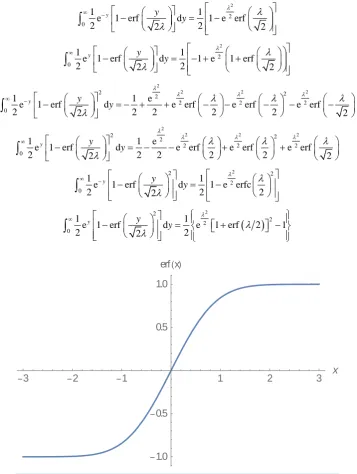
The following graph shown in Figure 1 represents the error function for x between −3 and +3. Linked to the function of errors, we have the complementary error function
( )
( )
erfc x = −1 erf x .
It can be easily seen that
( )
( )
erf − = −x erf x .
The calculation of the mean difference of the lognormal distribution requires the utilization of integrals in-volving various functions, one of these being the error function. These integrals, not available for consideration in standard mathematical calculation software, are presented here in forms rendered highly adaptable to various needs. In our adaptation, in order to obtain the mean difference of the lognormal model, these integrals have been listed as follows
2
2 0
1 1
e 1 erf d 1 e erf
2 2 2 2
y y
y
λ λ
λ
∞ −
− = −
∫
2
2 0
1 1
e 1 erf d 1 e 1 erf
2 2 2 2
y y y
λ λ
λ
∞
− = − + +
∫
2
2 2 2
2 2 2
2 2 2
0
1 1 e
e 1 erf d e erf e erf e erf
2 2 2 2 2 2 2
y y
y
λ
λ λ λ λ λ λ
λ
∞ −
− = − + + − − − − −
∫
2
2 2 2
2 2 2
2 2 2
0
1 1 e
e 1 erf d e erf e erf e erf
2 2 2 2 2 2 2
y y
y
λ
λ λ λ λ λ λ
λ
∞
− = − − + +
∫
2
2 2
2 0
1 1
e 1 erf d 1 e erfc
2 2 2 2
y y
y
λ λ
λ
∞ −
− = −
∫
(
)
2
2
2 2
0
1 1
e 1 erf d e 1 erf 2 1
2 2 2
y y y
λ
λ λ
∞
− = + −
[image:3.595.135.493.234.709.2]∫
Figure 1.Function of error for x between −3 and 3.
3 2 1 1 2 3
x
1.0 0.5 0.5 1.0
The first two integrals are easily calculated using mathematical software. The following two are very hard and were calculated considering particular cases of an integral given by Prudnikov, Brychkov and Marichev, 1986. The last two integrals were obtained by subtracting the first integral from the third, twice, and the second integral from the fourth, twice.
5. Calculation Procedure for the Mean Difference of Lognormal Distribution
To calculate the mean difference of lognormal distribution, it is possible to start from one of the four formulas indicated in paragraph 2. After several attempts, we opted for the formula based solely on the cumulative distri-bution function
( )
1( )
d baF x F x x
∆ =
∫
− .The cumulative distribution function of lognormal distribution, as indicated in paragraph 2, is
( )
1 log1 erf .
2 2 x F x λ = +
Utilizing the said cumulative distribution function in the Δ formula, after some simplifications, we obtain 2
0
1 log
1 erf d ,
2 2 x x λ ∞ ∆ = −
∫
introducing the transformation of the variable
log
Y = X,
we achieve the formula:
2 1
e 1 erf d ,
2 2
y y y
λ ∞ −∞ ∆ = −
∫
which, due to the symmetry of the error function, can also be expressed by the negative argument of the expo-nential function
2 1
e 1 erf d ,
2 2
y y y
λ ∞ − −∞ ∆ = −
∫
splitting the two integrals, we obtain the formulas
2 2
0
0
1 1
e 1 erf d e 1 erf d ,
2 2 2 2
y y y y
y y λ λ ∞ − − −∞ ∆ = − + −
∫
∫
2 2 0 0 1 1e 1 erf d e 1 erf d .
2 2 2 2
y y y y
y y λ λ ∞ −∞ ∆ = − + −
∫
∫
Considering the presence of equality
2 2
0
0
1 1
e 1 erf d e 1 erf d
2 2 2 2
y y y y y y
λ λ ∞ − −∞ − = −
∫
∫
,the formula for the mean difference can be expressed by utilizing only the integrals defined by the positive semi- axis
2 2
0 0
1 1
e 1 erf d e 1 erf d .
2 2 2 2
y y y y y y
The two integrals in this formula were obtained in the previous paragraph, introducing them into the said formula and simplifying, we obtain the extremely simple expression for the mean difference of the lognormal distribution:
(
)
2
2
2e erf 2 λ
λ
∆ = .
6. Conclusion
Through a painstaking process utilizing selected hard integrals with functions including the error function, we have obtained an extremely simple formula of the mean difference of the lognormal distribution. This result can be added to the other findings regarding other distribution models. This result is useful for elaborating in-depth characterizations of the lognormal model and facilitating comparisons with other variability indexes of the said model.
Attributions of Work
Girone Sections 2, 4 and 6, Manca Sections 1, 3 and 5.
References
[1] Girone, G. and Mazzitelli, D. (2007) La differenza media nei principali modelli distributivi continui, Annali del Dipartimento di Scienze Statistiche “Carlo Cecchi” dell’Università degli Studi di Bari, Cacucci Editore.
[2] Girone, G., Massari, A. and Mazzitelli, D. (2015) More on the Mean Difference of Continuous Distributive Models.
Spontaneous Contribution in the Proceedings/Book of Abstracts of the SIS Conference “Statistics and Demography:
The Legacy of Corrado Gini”, Treviso, 9-11 Settembre 2015.
[3] Girone, G., Manca, F. and D’Uggento, A.M. (2015) The Mean Difference of Discrete Distribution Models. Spontane-ous Contribution in the Proceedings/Book of Abstracts of the SIS Conference “Statistics and Demography: The Legacy of Corrado Gini”, Treviso, 9-11 Settembre 2015.