Export and Import Cointegration in Forestry Domain: The Case of Malaysia

Munich Personal RePEc Archive

Export and Import Cointegration in

Forestry Domain: The Case of Malaysia

Emmy, F.A. and Baharom, A.H. and Radam, Alias and

Illisriyani, I.

Universiti Putra Malaysia

4 August 2009

Online at

https://mpra.ub.uni-muenchen.de/16673/

Export and Import Cointegration in Forestry Domain: The Case of

Malaysia

by

F.A. Emmy*1, A.H Baharom2, Alias Radam1 and I. Illisriyani1

Abstract

This study was undertaken to explore the relationship between the export and import in the category of Forestry domain for Malaysia which includes sub domain (1)industrial roundwood; (2)wood pulp; (3)wood fuel; (4) paper and paper board; (5) sawn wood; (6) recovered paper and (7)wood base panel. Johansen (1991) cointegration method was employed and the period of the study covers monthly data from 1961 to 2007. The results clearly show that the export and import of forestry domain is highly cointegrated. Bi-directional granger causality could be detected based on VECM method. Imports seems to positively and significantly affect exports, both in the long run and short run, vice versa.

Key Words: Johansen cointegration test, forestry trade, VECM

Introduction

The forest products sector is estimated to contribute about one percent of world gross domestic product and account for three percent of international merchandise trade. As for the case of Malaysia, we produced an estimated 26.4 million cu m (932 million cu ft) of round wood from a forest area of 19.3 million ha (47.7 million acres) in 2000. About 32% of the forest area is located in Peninsular Malaysia, 22% in Sabah, and 46% in Sarawak. Exports of timber products in 2000 amounted to $3.8 billion, or 4.2% of total exports. Malaysia is the world's third leading producer (after Brazil and Slovakia) of veneer sheets, accounting for 7% of global production in 2000. While, forest products imports by Malaysia are dominated by paper products. In 1994 paper and paperboard comprised 83 percent of Malaysia's forest products imports. Malaysia, likewise Indonesia, is a major producer of hardwood forest products.

Numerous studies have flourished on the external imbalances in the current account. Most of these studies concentrated on aggregated trade imbalances, seldom have researches concentrated on the trade imbalances of a particular domain as what we are trying to attempt in this study, whereby we would like to focus on the trade imbalances in the category of Forestry domain. More precisely we intend to investigate the existence of any co-integrating factors between the export and import of the above category, if any. In the study of sustainability of external imbalances for 22 Least Developed Countries (LDC), Tang and Smyth (2008) found that the macroeconomic policies have been effective in causing the exports and imports to converge in the long run. It is a well known fact that much of the

1 _{Institute of Agricultural and Food Policy Studies, Universiti Putra Malaysia, 43400 UPM Serdang, Selangor,}

Malaysia.

* Corresponding author: emmyfarha@gmail.com

2 _{Department Economic, Faculty of Economics and Management, Universiti Putra Malaysia, 43400 UPM}

discussion in the empirical literature on external imbalances has focused on their sustainability.

.

The empirical literature that has examined the sustainability of external imbalances has adopted one of the two major empirical approaches. The first approach is to examine whether exports and imports are cointegrated, the same approach that we intend to employ in this study. The second approach to examine the sustainability of external imbalances is to test for a unit root in the current account. Using this method, if the current account or trade balance is found to be stationary, this implies that external imbalances are sustainable and that the international budget constraint is satisfied. If, however, the trade balance is non-stationary this is either a reflection of bad policies or indicative of the productivity gap hypothesis. To this point, the results in the empirical literature on the sustainability of external imbalances are mixed. Among the notable studies that followed the first approach are as those of Husted (1992), Bahmani-Oskooee (1994), Fountas and Wu (1999) and Irandoust and Ericsson (2004). Husted (1992) and Fountas and Wu (1999) used quarterly data for the periods 1967-1989 and 1967-1994 respectively, to examine whether exports and imports are cointegrated in the United States. While Fountas and Wu(1999) found no long-run relationship, Husted(1992) found that exports and imports were cointegrated. Employing quarterly data from 1971-1997, Irandoust and Ericsson (2004) found that exports and imports were cointegrated in Germany, Sweden and the United States. Bahmani-Oskooee (1994) found that Australian exports and imports are cointegrated, and the further concluded that the cointegrating coefficient was close to one, implying that Australia’s external account is sustainable. Using quarterly data, Bahmani-Oskooee and Rhee (1997) found that South Korea’s exports and imports are cointegrated and the coefficient on exports was positive. This result implies that South Korea does not violate its international budget constraint.

Employing the Gregory and Hansen (1996) cointegration test to examine the sustainability of external imbalances in Indonesia, Malaysia, the Philippines and Thailand, using annual data for the period, 1961-1999, Baharumshah et al. (2003) found that exports and imports are cointegrated in Indonesia, the Philippines, and Thailand, but not in Malaysia. In contrary, Tang (2002), employing bounds test for cointegration developed by Pesaran et al. (2001) to annual data for the period 1968-1998 (1974-1998 for Singapore) found cointegration between exports and imports for Malaysia and Singapore, but not for the Philippines, Indonesia and Thailand. Narayan and Narayan (2004) similarly employed the bounds test to examine long-run relationship between exports and imports in Fiji and Papua New Guinea and found that while exports and imports were cointegrated in both the countries, the coefficient on exports was equal to one, for only Fiji.

The purpose of this paper is to investigate the relationship between the export and import in the category of forestry domain which includes subdomains (1)industrial roundwood; (2)wood pulp; (3)wood fuel; (4) paper and paper board; (5) sawn wood; (6) recovered paper and (7)wood base panel. Johansen (1991) cointegration method was chosen to explore the probable cointegration. Vector error correction model (VECM) would be employed in the later stage to investigate the dynamic and long run relationship between these variables. Granger causality test based on VECM will also be conducted. Then the policy implication will be proposed which will benefit the sector itself and also the country.

Data and Methodology

The data used in this analysis are gathered from the Food and Agriculture Organization of The United Nations Statistical Database. The data was downloaded from the website faostat.fao.org. This study only focused on trade data for forestry domain namely, (1)industrial roundwood; (2)wood pulp; (3)wood fuel; (4) paper and paper board; (5) sawn wood; (6) recovered paper and (7)wood base panel in Malaysia over the period 1961 to 2007.

In empirical economics macroeconomic variables comprises of non stationary series. Treating non stationary variables in empirical analysis is important so that the results of spurious regression can be avoided. According to the concept of cointegration, two or more non-stationary time series share a common trend, then they are said to be cointegrated. The theoretical framework highlighted are expressed as follows: the component of the vector Yt = (y1t,y2t,…,ynt)’ are considered to be cointegrated of order d,b, denoted Yt ~ CI (d,b) if (i) all the component Yt are stationary after n difference, or integrated of order d and noted as Yt ~ I(d). (ii) presence of a vector = ( 1, 2,…, n) in such that linear combination Yt = 1y1t + 2y2t +…+ nynt whereby the vector is named the cointegrating vector. A few major characteristics of this model are that the cointegration relationship obtained indicates a linear combination of non-stationary variables, in which all variables must be integrated of the same order and lastly if there are n series of variables, there may be as many as n-1 linearly independent cointegrating vectors.

Johansen’s (1991) cointegration test is adopted to determine whether the linear combination of the series possesses a long-run equilibrium relationship. The numbers of significant cointegrating vectors in non-stationary time series are tested by using the maximum likelihood based trace and max statistics introduced by Johansen and Juselius (1990). The advantage of this test is that it utilises test statistic that can be used to evaluate cointegration relationship among a group of two or more variables. Therefore, it is a superior test as it can deal with two or more variables that may be more than one cointegrating vector in the system.

Prior to testing for the number of significant cointegrating vectors, the likelihood ratio (LR) tests are performed to determine the lag length of the vector autoregressive system. In the Johansen procedure, following a vector autoregressive (VAR) model, it involves the identification of rank of the n x n matrix in the specification given by:

t k t k

i

i t i

t Y Y

Y =δ+ Γ∆ +∏ +ε

∆ −

−

= −

1

1

(1)

where Yt is a column vector of the n variables, is the difference operator, and are the coefficient matrices, k denotes the lag length and is a constant. In the absence of cointegrating vector, is a singular matrix, which means that the cointegrating vector rank is equal to zero. On the other hand, in a cointegrated scenario, the rank of could be anywhere between zero. In other words, the Johansen cointegration test can determine the number of cointegrating equation and this number is named the cointegrating rank.

+ = ∧ − − = p r i trace r T

1 ) 1 ln( ) ( λ λ (2) + = + ∧ − − = + p r i r trace r r T

1 1) 1 ln( ) 1 , ( λ

λ (3)

where p is the number of separate series to be analysed, T is the number of usable observations and is the estimated eigenvalues.

Vector Error Correction Model (VECM)

VECM is a restricted VAR designed for use with non stationary variables that are known to be co-integrated. VECM specification restricts the long run behaviour of the endogenous variables to converge to their co-integrating relationships while allowing for short-run adjustment dynamics. Engle and Granger (1987) showed that if the variables, say Xt and Yt is found to be cointegrated, there will be an error representatives which is linked to the said equation, which gives the implication that changes in dependent variable is a function of the imbalance in cointegration relation (represented by the error correction term) and by other explanatory variables. Intuitively, if Xt and Yt have the same stochastic trend, current variables in Xt (dependent variable) is in part, the result of Xt moving in line with trend value of Yt (independent variable). Through error correction term, VECM allows the discovery of Granger Causality relation which has been abandoned by Granger (1968) and Sims (1972). The VAR constraint model may derive a VECM model as shown below:

= − = − + ∆ + ∆ + =

∆ δ ρ θ ρ φ ε

1 1 0 i t i t i i i t i

t y x

y

where yt – in the form of n x 1 vector

i and i– estimated parameters

– difference operator

t – reactional vector which explains unanticipated movements in

Yt and x (error correction term)

In the Granger causality test, the degree of exogeneity can be identified through the t test for the lagged error correction term ( i), or F test applied to the lags of the coefficients of each

variable separately of the non dependent variable ( i). In addition to the above, VECM method allows the differentiation of the short term and long term relationship. Error term with lagged parameter (ECT (e1, t-1)) is an adaptive parameter where it measures the short term

Empirical Result

Table 1 reports the results of Augmented Dickey-Fuller (ADF) and Phillips-Perron (PP) unit root test that describes the stationary properties of the variables (export and import) in Malaysia. Schwartz Information Criterion (SIC) is used to select the optimal truncation lag length to ensure the errors are white noise in ADF. The both results clearly show that the null hypothesis of unit root test for all variables fail to be rejected in the level form but only appear stationary in the first different. In other words, all variables are said to be integrated of order one, which is I(1).

Table 1:Results of the Unit Root Tests

ADF PP

Level First Different Level First Different Variables

(Trend and Intercept)

(Trend and Intercept)

(Trend and Intercept)

(Trend and Intercept) Export -1.5571

(0)

-6.9264*** (1)

-1.4166 -8.4279***

Import -2.6017 (0)

-7.8283*** (0)

-2.5829 -7.8325***

Note: ** denotes significant at 1% level. Figures in parenthesis ( ) refer to the selected length. The lag length was arbitrarily selected using SIC.

Since all the variables are integrated of same order, the cointegration test is conducted to determine the presence of a long run equilibrium relationship between export and import in the categories of forestry domain. The results of Johansen cointegration test is reported in Table 2. The results indicate that null hypothesis of no cointegration can be rejected in the period. Therefore, it can be concluded that there is positive and significant long run relationship at one percent level, implying that there is common trend exists within import and export.

Table 2: Results of Cointegration Test

Vectors r=0 r 1

Trace test 20.38 4.37 1% level 20.04 6.65 Max-Eigen test 16.01 4.37 1% level 18.63 6.65

Note: r indicates the number of cointegrating vectors. Trace and Max-Eigen denote the trace statistic and maximum eigenvalue statistic. The critical values obtained from Osterwald-Lenum (1992). Lag selection (k) is based on Schwert (1987) formula.

Table 3: Long-run elasticities

Independent Variables Dependent Variables

ln Im ln Ex ln Im 3.31*** (-6.22) ln Ex 0.30** (-2.45)

Note: * and ** denote significant at 10% and 5% levels respectively. t-stats in parentheses.

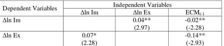
Table 4: Short-run elasticities

Independent Variables Dependent Variables

ln Im ln Ex ECMt-1

ln Im 0.04**

(2.97)

-0.02** (-2.28) ln Ex 0.07*

(2.28)

-0.14** (-2.93)

Note: * and ** denote significant at 10% and 5% levels respectively. t-stats in parentheses.

Conclusion

In this study, the Johansen cointegration test is employed to test the relationship between export and import in categories of forestry domain. The sample period of study was 1961 to 2007 using annual data. All the data went through log-log transformation so that the estimates will be less sensitive to outliers or influential observations and also order to reduce the data range. From the analysis, we found that the import and export in the forestry domain is cointegrated, a finding concurrent with a number of past studies such Husted (1992), Irandoust and Ericsson (2004), Bahmani-Oskooee (1994), Baharumshah et al. (2003) and Narayan and Narayan (2004) to name afew. There exist significant and positive both dynamic and long-run relationship between both variables. Based on VECM, bidirectional granger causality could be detected among the variables. From a policy point of view, restricting imports in the forestry domain could backfire and could turn out to be harmful for the Malaysian economy. Policy makers should be cautious in implementing any trade inflow policies in the domain of forestry.

References

Baharumshah A Z, Lau E and Fountas S (2003). On the Sustainability of Current Account Deficits: Evidence from Four ASEAN Countries, Journal of Asian Economics, Vol. 14, No.3, pp. 465-487.

Bahmani-Oskooee M (1994). Are Imports and Exports of Australia Cointegrated?, Journal of Economic Integration, Vol. 9, No. 4, pp. 525-533.

Bahmani-Oskooee M and Rhee H J (1997). Are Imports and Exports of Korea Cointegrated?,

International Economic Journal, Vol. 11, No. 1, pp. 109-114.

Engle, R.F. and Granger, C.W.J. (1987). Cointegration and error correction: representation, estimation, and testing, Econometrica, 55, 251 – 276.

Fountas S and Wu J L (1999). Are the US Current Account Deficits Really Sustainable?,

Irandoust M and Ericsson J (2004). Are Import and Exports Cointegrated? An International Comparison, Metroeconomica, Vol. 55, No. 1, pp. 49-64.

Johansen, S. (1991). Estimation and hypothesis testing of cointegration vectors in Gaussian vector autoregressive models, Econometrica 59, 1551–1580.

Johansen, S. and Juselius, K. (1990). The full information maximum likelihood procedure for inference on cointegration—with applications to the demand for money. Oxford Bulletin of Economics and Statistics,52, 169–210.

Narayan P K and Narayan S (2004). Are Exports and Imports Cointegrated? Evidence from Two Pacific Island Countries, Economic Papers, Vol. 23, No. 2, pp. 152-164.

Puah, C.H,. Sze-Wei, Y., Mansor, S.A and Lau, E (2008) Exchange rate and trade balance nexus in Asean-5, Labuan Bulletin of International Business and Finance, 6, 19-37.

Tang T.C (2002). Are Imports and Exports of the Five ASEAN Economies Co-integrated? An Empirical Study, International Journal of Management, Vol. 20, pp. 88-91.