Modeling of Imperfect Data in Medical Sciences by Markov Chain with Numerical Computation

http://dx.doi.org/10.4236/abb.2014.513114

How to cite this paper: Afshari, M. and Ghaffaripour, A. (2014) Modeling of Imperfect Data in Medical Sciences by Markov Chain with Numerical Computation. Advances in Bioscience and Biotechnology, 5, 1003-1008.

http://dx.doi.org/10.4236/abb.2014.513114

Modeling of Imperfect Data in Medical

Sciences by Markov Chain with Numerical

Computation

Mahmoud Afshari1*, Anoshirvan Ghaffaripour2

1_{Department of Statistics, College of Science, Persian Gulf University,Bushehr, Iran} 2_{Department of Statistics, College of Science, Yasouj University, Yasuj, Iran}

Email: *[email protected]

Received 24August 2014; revised 7October 2014; accepted 1November 2014

Academic Editor: Jisook Kim, University of Tennessee at Chattanooga, USA

Copyright © 2014 by authors and Scientific Research Publishing Inc.

This work is licensed under the Creative Commons Attribution International License (CC BY). http://creativecommons.org/licenses/by/4.0/

Abstract

In this paper we consider sequences of observations that irregularly space at infrequent time in-tervals. We will discuss about one of the most important issues of stochastic processes, named Markov chains. We would reconstruct the collected imperfect data as a Markov chain and obtain an algorithm for finding maximum likelihood estimate of transition matrix. This approach is known as EM algorithm, which includes main optimum advantages among other approaches,

and consists of two phases: phase (maximization of target function). Continue the phase E and M to achieve the sequence convergence of matrix. Its limit is the optimal estimator. This

algo-rithm, in contrast with other optimum algorithms which could be used for this purpose, is practi-cable in maximum likelihood estimate, and unlike to the methods which involve mathematical, is executable by computer. At the end we will survey the theoretical outcomes with numerical com-putation by using R software.

Keywords

Markov Chain, Matrix Transition, Maximum Likelihood, EM Algorithm, Missing Data

1. Introduction

Today, we humans are faced with many of the random variables and processes. One of the most important issues

is the random process of Markov chain. Markov chain is often used to describe how the system changes over time. If we are able to model the system sufficiently to form a Markov chain model, we can then evaluate its various theoretical results through system analysis. In this article, the Matrix transition of Markov chain needed for imperfect observation within a given time is obtained through EM algorithm.

The EM algorithm has two stages: E stage and M stage. This algorithm basically works in this way: We first take into consideration the initial value for the parameter which in this case is the transition matrix.

The full set of data (X) is then reconstructed from missing data by estimation of these parameters in E

stage. In the M stage, the maximum likelihood of reconstructed data is maximized to get a new estimation of the parameter. Then, based on this new estimation, the E stage is repeated and we get the second estimation in the M stage. Finally, we continue this process as far as to get convergence estimates.

Dempstr [1], Raj [2], Johnson et al. [3] have obtained the value of maximum likelihood of the transition ma-trix for a sequence of observations.

Among the researchers who examined the issues of statistical inference of Markov chains and published arti-cles in this area are Melichson [4], Capee [5], Chip [6] and Robert [7].

2. Modeling of Missing Data Based on Markov Chain

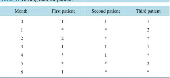
Following observations inTable 1 are series of real data obtained about a kind of disease related to 3 patients at different times during 6 months in a hospital. We have missed some of the data because the patients have not at-tended the hospital in some cases. Number 1 indicates that the patient’s condition is satisfactory and number 2 shows the patients are in a very bad condition. The asterisk indicates that in a particular time point, the data has not been observed.

First, the patient’s condition is reported as: 1) Next month, no data are is available. Two months later the con-dition of that patient is reported as; 2) One month later his concon-dition is reported as (1) again, and so on. We call such a set of data incomplete and it is shown as Y.

The incomplete data are collected against complete data (X) which are gathered in all intervals between the first and the last observation.

Such a system can be modeled as a Markov chain with E condition space and transition matrix P.

Generally, we will have X =Nij if we consider Oijt as the number of condition change from i to j at the

time interval t. Pijk as the transition probability from i to j condition at t time, Nij as the number of

con-dition change from i to j in a time unit for the whole X data , and

( )

r ij

P as the element of matrix r

P , i.e. condition change probability r a stage from i to j condition. Having this fact in mind that with the incom-plete data Y and the nonzero suitable initial transition matrix, there will be different complete data X with their own probabilities, we estimate the transition matrix by the EM algorithm as follows:

1—First, we change the specified incomplete data (Y) to complete data (X) by considering a suitable amount for those intervals we have no observation and data. In other words, we reconstruct the complete data (X) from the incomplete data.

2—We consider an initial value for an arbitrary non-zero element of the transfer matrix as P( )0.

[image:2.595.172.456.588.718.2]

3—We compute maximum likelihood of X observations with the initial transmission matrix P( )0 as fol-lows:

Table 1. Missing data for patient.

Month First patient Second patient Third patient

0 1

1 *

2 2

3 1

4 *

5 *

6 1

1

*

*

1

1

*

*

1

2

*

1

*

2

( )

(

0

)

( )

( )

( )

( )

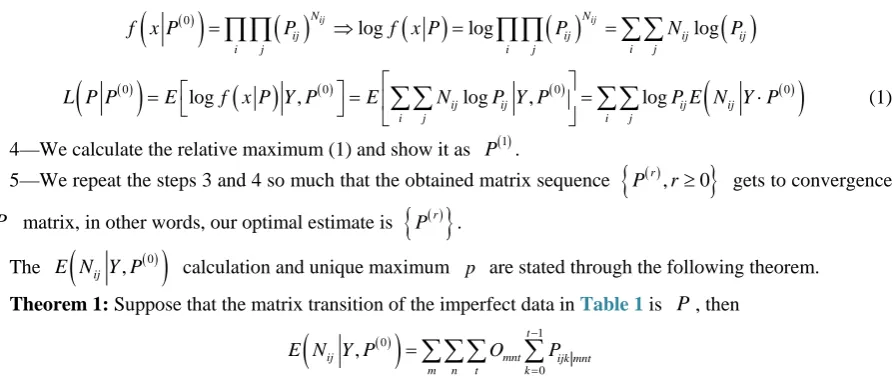
log log log

ij ij

N N

ij ij ij ij

i j

i j i j

f x P =

∏∏

P ⇒ f x P =

∏∏

P =

∑∑

N P

( )

(

0

)

( )

( )0 ( )0

(

( )0

)

log , ijlog ij , log ij ij

i j i j

L P P =E_ f x P Y P _=E_ N P Y P _= P E N Y P⋅



∑∑



∑∑

(1)

4—We calculate the relative maximum (1) and show it as P( )1.

5—We repeat the steps 3 and 4 so much that the obtained matrix sequence

{

P( )r ,r≥0

}

gets to convergence

P matrix, in other words, our optimal estimate is

{ }

P( )r .

The E N Y P

(

ij , ( )0

)

calculation and unique maximum p are stated through the following theorem.

Theorem 1: Suppose that the matrix transition of the imperfect data inTable 1 is P, then

( )

(

)

1

0

0 ,

t

ij mnt ijk mnt

m n t k

E N Y P O P

−

=

=

∑∑∑

∑

Proof: We assume the system at the time t0 is in the m condition and at the next time interval it is in the n condition. The probability that a change occurs between conditions i and j is done in the k time in-terval is computed according to the Figure 1 provided that the system gets to n condition at t0+t from the

starting point condition m at t0.

First the system starting from m condition changes to i condition with the probability of

( )

k

mi

P at the time unit of k. Then the system is likely to change to n condition at t0+t with the probability of

(

)

1 l k

jn

P− − . Suppose that we define A and B as follows:

A: Cases in which changes from i to j condition occurs at t0+t.

B: Cases in which system starting from m condition at t0 gets to n condition at t0+t.

Then we have:

( )

(

_{( )}

)

( ) (

_{( )}

)

( )

1 0

.

0 1, 1,

k t k

ij

mi jn

ijk mnt _t

mn

P P P

P A B

k t P P P A B

P B _P

− −

≤ ≤ − = = =  =

It is clear that the probability of the number of condition changes between the i and j conditions along with a change from m to n condition at the t time interval is equal to:

1

0 t

ijk mnt k

P

−

=

∑

.

So, the expected number of such condition changes in all time intervals is:

1

0 t

mnt ijk mnt k

O P

−

=

∑

because m and

n conditions repeatedly occurs at t intervals. Therefore, the expected number of transitions from i to j

condition on the condition of observed data Y and Matrix transition P accumulating on all observed data is obtained as follows:

(

( )

)

1 0

0 ,

t

ij mnt ijk mnt

m n t k

E N Y P O P

−

=

=

∑∑∑

∑

.

Theorem 2: Suppose that the matrix transition of the imperfect data inTable 1 is P, then there is a unique relative maximum with its entry is as follows:

( )

(

)

( )

(

)

,

, 0

r ij

ij _r

ij j

E N Y P P

E N Y P

=

≠

[image:3.595.92.540.82.270.2]

∑

Proof: ( )

(

)

( )

(

)

(

( )

)

( )

(

)

(

( )

)

1 1 1 2 1 1

1 2 2

, log

, log , log

, log , log 1

r

P ij ij

i j

r r

ij ij i i

i j i

r r

ij ij i i

i j i i

Q E N Y P P

E N Y P P N Y P P

E N Y P P N Y P P

= = = = =   =       = _ + _      = _ + _ − _    

∑∑

∑∑

∑

∑∑

∑

∑

(2)

Equation (2) has been obtained because the sum of entries in each line is one.

( )

(

)

( )

( )

( ) ( ) 1 1 1 1 2

, ₁ , ,

, 1

r r r

ij _r ij i

P

i

ij ij ij i

i i

N Y P N Y P N Y P

Q

E N Y P E

P P P P

P ∞ =      ₋  ∂ _{=  +  =  − }     ∂  ₋      

∑

 ( ) ( ) 1 1 , , 0 r r ij i P

ij ij i

E N Y P E N Y P

Q

P P P

    ∂ _{= ⇒}   ₌   ∂ ( ) ( ) 1 1 , , ij i r r ij i P P

E N Y P E N Y P

⇒ =

   

   

(3)

Adding Equation (3) on i, we have:

( ) ( ) 1 1 , , r i i r ij j

E N Y P P

E N Y P

 

 

=

 

 

∑

(4)

By replacing Equation (4) in Equation (3), the proof is completed.

Remark: the fourth stage in algorithm is computed and algorithm is completed as the following:

1) We compute

(

( )

)

1 0

0 ,

t

ij mnt ijk mnt

m n t k

E N Y P O P

−

=

=

∑∑∑

∑

.

2) We compute matrix transition of first stage through this formula:

( )

(

)

( )

(

)

0 0 , , 0 ij ij ik k

E N Y P P

E N Y P

=

≠

∑

The obtained Pijs for all i and j forms another matrix in the form of

( )1

P for the next iteration.

3. Numerical Computation

In this section, all the theories mentioned are surveyed on the Table 1 through a program written in R soft-ware.

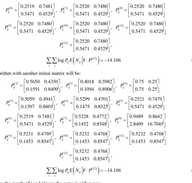
For actual observations we haveTable 2 which is number of change from i to j at the time interval t. Conducting computer program written on the bases of the EM algorithm to estimate the matrix transition of the system and the original transition Pij( )0 , we will have the following outputs:

( )2 0.2483 0.7517

0.5512 0.4488

ij

P =  _

 ,

( )1 0.2509 0.7491

0.5206 0.4794

ij

P =  _

 ,

( )0 0.333 0.667

0.667 0.333

ij

P =  _

 

( )3 0.2534 0.7466

0.5464 0.4536

ij

P =  _

 ,

( )4 0.2515 0.7485

0.5472 0.4528

ij

P =  _

 ,

( )5 0.2521 0.7479

0.5471 0.4529

ij

P =  _

( )6 0.2519 0.7481

0.5471 0.4529

ij

P =  _

 ,

( )7 0.2520 0.7480

0.5471 0.4529

ij

P =  _

 ,

( )8 0.2520 0.7480

0.5471 0.4529

ij

P =  _

 

( )9 0.2520 0.7480

0.5471 0.4529

ij

P =  _

 ,

( )10 0.2520 0.7480

0.5471 0.4529

ij

P =  _

 ,

( )11 0.2520 0.7480

0.5471 0.4529

ij

P =  _

 

( )12 0.2520 0.7480

0.5471 0.4529

ij

P =  _

 ,

( )

(

12

)

log ij ij 14.106

i j

P E N Y P⋅ = −

∑∑

(5)

EM Algorithm with another initial matrix will be:

( )2 0.5650 0.4350

0.1591 0.8409

ij

P =  _

 ,

( )1 0.4018 0.5982

0.1094 0.8906

ij

P =  _

 ,

( )0 0.75 0.25

0.75 0.25

ij

P =  _

 

( )3 0.5059 0.4941

0.1397 0.8603

ij

P =  _

 ,

( )4 0.5299 0.4701

0.1475 0.8525

ij

P =  _

 ,

( )5 0.2521 0.7479

0.5471 0.4529

ij

P =  _

 

( )6 0.2519 0.7481

0.5471 0.4529

ij

P =  _

 ,

( )7 0.5228 0.4772

0.1452 0.8548

ij

P =  _

 ,

( )8 0.9489 0.8642

2.8409 16.7045

ij

P =  _

 

( )9 0.5231 0.4769

0.1453 0.8547

ij

P =  _

 ,

( )10 0.5232 0.4768

0.1453 0.8547

ij

P =  _

 ,

( )11 0.5232 0.4768

0.1453 0.8547

ij

P =  _

 

( )12 0.5232 0.4768

0.1453 0.8547

ij

P =  _

 ,

( )

(

12

)

log ij ij 14.106

i j

P E N Y P⋅ = −

∑∑

(6)

As it is seen, the results (5) and (6) are the same in either way.

4. Conclusions

In using the EM algorithm, we are practically faced with some issues which should be focused to accelerate our work and save time.

1) If the initial transition matrix P( )0 , which is arbitrarily chosen, is of a zero entry or the number of transi-tions from one condition to another one is zero in a unit of time, the corresponding entries of all produced ma-trices are zero, too. The initial matrix entries must be non-zero to avoid such condition.

[image:5.595.141.528.80.447.2]

2) Increase in the number of time units between successive observations increases the power of transition ma-trix. If the number of the observed condition changes is relatively low, the time interval between observations is high. Accordingly, with respect to time needed for computation, it is not economical to integrate all these to-

Table 2. Condition change from i to j at the time interval t for miss-ing data.

ijt

O : number of condition change from i to j at the time t

Time 1 2 3 4 5 6

11

O 1 * 4 1 * 1

12

O 1 2 * * 1 *

21

O 1 4 * 1 * *

22

gether in the analysis. Actually it is better to keep the maximum time interval at the level in which the probabil-ity of condition change is ignored. If the maximum time interval is too large, the increase in the time unit can be effective.

3) If the maximum time intervals are relatively low, the computation time of each stage is short, although dif-ferent performances may be necessary before achieving convergence.

4) In practical computation, we have accepted that when the maximum difference between successive entries of transition matrix is smaller than a predetermined value, e.g. ε=10−4. In other words, convergence is achieved when for all values of i, j, and the given value for r, we have: Pij( )r 1 Pij( )r ε

+ _{− <}

.

Acknowledgements

The support of Research Committee of Persian Gulf University is greatly acknowledged.

References

[1] Dempstr, A.P., Larid, N.M. and Rubin, D.B. (1997) Maximum Likelihood from Incomplete Data via the EM Algo-rithm. Journal of the Royal Statistical Society, 39, 1-38.

[2] Raj, B. (2002) Asymmetry of Business Cycles: The Markov-Switching Approach, Soft-Tissue Material Properties Un-der Large Deformation: Strain Rate Effect. Hand Book of Applied Econometrics and Statistical Inference, 3, 687-710. [3] Johnson, C. and Gallivan, S. (1995) Estimating a Markov Transition Matrix from Observational Data. Journal of the

Operational Researches Society, 46, 405-410.http://dx.doi.org/10.1057/jors.1995.55

[4] Melichson, I. (1999) A Fast Improvement to the EM Algorithm on the Own Terms. Journal of the Royal Statistical

So-ciety—Series B, 51, 127-138.

[5] Cappee, O., Moulines, E. and Ryden, T. (2005) Inference in Hidden Markov Models. Springer, New York.

[6] Chib, S. (1996) Calculating Posterior Distributions and Modal Estimates in Markov Mixture Models. Journal of Eco-

nometrics, 75, 79-97.http://dx.doi.org/10.1016/0304-4076(95)01770-4

[7] Roberts, W. and Ephraim, Y. (2008) An EM algorithm for Ion Chanel Current Estimation. IEEE Transactions on