Air Pollution Prediction via Differential Evolution Strategies with Random Forest Method

© 2017, IRJET | Impact Factor value: 6.171 | ISO 9001:2008 Certified Journal

| Page 1083

Air pollution prediction via Differential evolution strategies with

random forest method

---***---Abstract –

concentration of C6H6, NO2, O3, SO2, CO, PM2.5 and PM10 are of great importance to protect human health and control air pollution. In this paper, we infer air quality data from Central Pollution Control Board India of two cities Delhi and Patna. Existing independent classifier of Bayesian network can be used to estimate the probability of an air pollutant and multi-label classifier which simultaneously predict multiple air pollutants. We compared the performance of the independent and multi-label classifier to the differential evolution strategies with random forest method which is an ensemble based method gaining popularity in prediction. Instead of focusing on single technique we are proposing hybrid technique by combining differential evolution with random forest. Our approach validate experimentally that it leads to performance gains when compared with independent classifier of Bayesian networks and multi-label classifier techniques based on four parameters i.e. accuracy, area under curve, success index and correlation.

Key Words: Air pollution prediction, Independent classifier, Multi-label classifier, Differential evolution, Random forest.

1. INTRODUCTION

In addition to land and water, air is the prime resource for sustenance of life. Clean air is the basic need of every living being. Air pollution is one of the major issues that have been affecting human health, agricultural crops, forest species and ecosystems. Exposure to air pollution has been associated with morbidity and mortality. Polluted air has adverse effects on entire nature and living organisms. Variety of air pollutants are emitted into the atmosphere by natural and anthropogenic sources, out of which particulate matters, sulphur dioxide, ozone, nitrogen dioxide, benzene and carbon monoxide are having the significant adverse impact on air quality.

An air pollutant is a substance in the air that can have adverse effects on humans and the ecosystem. The substance can be solid particles, liquid droplets, or gases. A pollutant can be of natural origin or man-made. Pollutants are classified as primary or secondary. Primary pollutants are usually produced from a process, such as

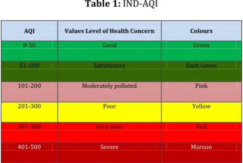
carbon monoxide gas from motor vehicle exhaust, or the sulphur dioxide released from factories. Secondary pollutants are not emitted directly. Rather, they form in the air when primary pollutants react or interact. Ground level ozone is a prominent example of secondary pollutant [20]. Real-time air quality information, such as the concentration of C6H6, NO2, O3, SO2, CO, PM2.5 and PM10 is of great importance to support air pollution control and protect humans from damage by air pollution. Traditionally, air quality status has been reported through voluminous data. Thus, it was important that information on air quality is put up in public domain in simple linguistic terms that is easily understood by a common person. Air Quality Index (AQI) is one such tool for effective dissemination of air quality information to people [26]. An air quality index is defined as an overall scheme that transforms the weighed values of individual air pollution related parameters (for example, pollutant concentrations) into a single number or set of numbers. As the AQI increases, an increasingly large percentage of the population is likely to experience increasingly severe adverse health effects. To compute the AQI requires an air pollutant concentration from a monitor or model. The function used to convert from air pollutant concentration to AQI varies by pollutants, and is different in different countries. Air quality index values are divided into ranges, and each range is assigned a descriptor and a colour code. In this paper, we use Indian National Air Quality Standard (INAQS) issued for 12 parameters [(carbon monoxide (CO), nitrogen oxide (NO2), sulphur dioxide (SO2), particulate matter (PM) of less than 2.5 microns size (PM2.5, PM of less than 10 microns size (PM10), ozone (O3), lead (Pb), ammonia (NH3), benzo(a)Pyrene (BaP), benzene (C6H6), arsenic (As), and nickel (Ni)] as shown in Table 1. An expert committee was constituted with members drawn from academia, medical fraternity, research institutes, Ministry of Environment and Forest (MoEF), advocacy groups, and Central Pollution Control Board (CPCB) [29]. The committee was mandated to deliberate, discuss and devise consensus on the AQI system that is appropriate for Indian conditions.

Rubal

© 2017, IRJET | Impact Factor value: 6.171 | ISO 9001:2008 Certified Journal

| Page 1084

AQI Values Level of Health Concern Colours

0-50 Good Green

51-100 Satisfactory Dark Green

101-200 Moderately polluted Pink

201-300 Poor Yellow

301-400 Very poor Red

401-500 Severe Maroon

There are six AQI categories, namely Good, Satisfactory, Moderately polluted, Poor, Very Poor, and Severe. We consider the dataset publically made available by Central Pollution Control Board (CPCB) India [27]. It contains data regarding two stations Delhi and Patna. The following variables measured at Delhi station: NO2, CO and Benzene. The station Patna measured following variables: PM2.5, PM10, SO2 and Ozone.

In this context, we explore the usage of Differential algorithm in air pollution prediction. The Differential Evolution (DE) method was developed by Price and Storn in 1996. It is a simple and fast, population based stochastic function minimizer. DE optimizes a problem by maintaining a population of candidate solution and creating new candidate solution by combining existing ones according to its simple formulae, and then keeping whichever candidate solution has the best score or fitness on the optimization problem. In this way the optimization problem is treated as black box that merely provides a measure of quality given a candidate solution [28]. In general, the random forest is an ensemble method that combines the prediction of several decision trees. In the random forest approach, a large number of decision trees are created. Every observation is fed into every decision tree. The most common output for each observation is used as the final output.

The rest of the paper is organized as follows. Section 2 gives the related work. Section 3 proposes Differential evolution strategies with random forest method and prediction of various gases in Delhi and Patna. Experiments are discussed in Section 4 followed by the results. Finally, this paper is concluded in Section 5.

2. RELATED WORK

Air pollution prediction is a prevalent research topic in the literature. Muhammad Atif Tahir et al (2011) they shows multi-label classification is a challenging research problem

in which each instance may belong to more than one class. The aim of this paper was to use heterogeneous ensemble of multi-label learners to simultaneously tackle both the sample imbalance and label correlation problems [21]. Patricio Perez (2012) [6] represented the results of a PM10 forecasting model that has been applied for air quality management in Santiago and Chile. The daily operation of this model has served to inform in advance to the population about the air quality and to help environmental authorities in the decision to take actions on days when concentrations are in ranges considered significantly harmful. In 2013, Yu Zheng et al [3] represented the real-time and fine-grained air quality information throughout a city, based on the air quality data reported by existing monitor stationsand a variety of data sources observed in the city, such as meteorology, traffic flow, human mobility, structure of road networks, and point of interests (POIs). Then they proposed a semi-supervised learning approach based on a co-training framework that consists of two separated classifiers. One is a special classifier and the other is a temporal classifier.

© 2017, IRJET | Impact Factor value: 6.171 | ISO 9001:2008 Certified Journal

| Page 1085

namely spatially averaged wind speed and wind direction. These factors are selected according to correlation and importance measures. Then the random forest method was proposed to build an hour-ahead wind power predictor.

3. DIFFERENTIAL EVOLUTION WITH RANDOM

FOREST METHOD

This paper proposes the process of predicting air pollutants via Differential evolution method with random forest. The challenges of our approach lie in two aspects. The first is to identify discriminative features from two different cities. The second one is how to incorporate heterogeneous features into a data analytics model effectively. We train the classifiers using training set, tune the parameters using validation set and then test the performance of classifiers on unseen test set. Also, our approach evaluated using dataset consisting of C6H6, NO2, O3, SO2, CO, PM2.5 and PM10 concentrations of Delhi and Patna.

3.1

Differential Evolution

DE is an Evolutionary algorithm. In the DE algorithm [23], each vector xGi,j consists of D variables xGi,j in the range [xmin(j), xmax(j)] , j = 1,….,D. The initial population should

more effectively cover the entire search space as much as possible by uniformly randomized individuals with search space constrained using the prescribed minimum and maximum parameter bounds. Initial vectors are randomly generated. We can initialize the jth parameter in the ith decision vector at the generation as follows:

X0i,j = xmin(j) + randi,j(0,1). (xmax(j) – xmin(j)), j = 1,….,D

Where randi,j(0,1), represents a uniformly distributed

random variable within the range [0,1].

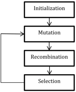
The process of Differential Evolution is illustrated in Fig. 1, the process is divided into four steps:

a) Initialization: - The DE algorithm randomly selects the initial parameter value uniformly on the intervals. Also initialization defines upper and lower bounds for each parameter.

b) Mutation Operation: - In the DE algorithm, mutation is a random change of the population to approach a favourable solution in the search space. Mutation expands the search space. The parent vector in the DE algorithm is mutated into mutant vector V. The algorithm employs mutation operation to produce a mutant (donor) vector with respect to each individual.

c) Recombination Operation: - Recombination incorporates successful solution from the previous generation. The trial vector is developed from the elements of the target vector and the elements of the mutant (donor) vector according to a predefined probability. Recombination reuses previously successful individuals.

d) Selection Operation: - Selection operation decides whether the target (parent) or trial vector survives into the next generation. The objective function value of each trial vector is compared with that of its corresponding target vector in the current population. If the trial vector yields lower objective function value compared with the corresponding target vector, the trial vector replaces the target vector and enters the population of the next generation. Otherwise, the target vector is retained in the population into the next generation.

Fig 1: Differential Evolutionary Algorithm Procedure

3.2 Random Forest

In recent years, decision trees have become a very popular machine learning technique because of its simplicity, ease of use and interpretability [15]. There have been different studies to overcome the shortcomings of conventional decision trees, e.g. their suboptimal performance and lack of robustness. One of the popular techniques that resulted from these works is the creation of an ensemble of trees followed by a vote of most popular class labelled forest. Random forest is one of the most successful ensemble learning techniques which have been proven to be very popular and powerful techniques in the pattern recognition and machine learning for high dimensional classification and skewed problems. The basic principle is called bagging (bootstrap aggregation), where a sample of size n taken from the training set Sn is selected randomly and fitted to a regression tree. This sample is called bootstrap, and it is chosen by replacement, which means

Initialization

Mutation

Recombination

© 2017, IRJET | Impact Factor value: 6.171 | ISO 9001:2008 Certified Journal

| Page 1086

that the same observation (Xi, Yi) may appear several times [24]. The main advantage of bootstrap aggregation is immunity to noise, since it generates non correlated trees through different training samples. The two main characteristics distinguish the random forest: -

a) Out-of-bag error: - The out-of-bag error OOBE, also called generalization error, is a kind of built in cross validation. It is the average prediction error of first-seen observations, i.e. using only the trees that did not see these observations while training. More explicitly, for each observation (Xi, Yi) of Sn, estimation is achieved by aggregating only the trees constructed over bootstrap samples not containing (Xi, Yi).

b) Variable importance: - The variable importance VI measure is obtained by permuting a feature andaveraging the difference in OOBE before and after permutation over all trees. If permutations over the variable lead to increase error, this variable is relevant. The more the score increases, the more the variable becomes important.

3.3 Algorithm

Input : Actual data, Population size, Crossover rate

Output : Predicted data

STEP 1. Read data and divide it into training and testing

STEP 2. Deploy differential evolution strategy to initialize population of candidate solution

STEP 3. Apply mutation and recombination for creating new candidate solution by combining the existing ones

STEP 4. Evaluate fitness value

STEP 5. If (new value < existing value) Then

Select the new value Else

Discarded and process starts from mutation

STEP 6. Apply random forest method

STEP 7. Get the predicted pollutants

STEP 8. End

3.4 Predicting CO, NO2 and Benzene in Delhi

The study area is Punjabi Bagh station in the city Delhi. We consider dataset which is publically made available by Central Pollution Control Board (CPCB) India. It contains data regarding a station Punjabi Bagh [30]. The following

variables are measured at this station: CO air quality index, NO2 air quality index, Benzene air quality index, temperature, humidity, wind speed and wind direction. Carbon monoxide (CO) is an important criteria pollutant which is ubiquitous in urban environment. CO production mostly occurs from sources having incomplete combustion. Due to its toxicity and appreciable mass in atmosphere, it should be considered as an important pollutant in AQI scheme. This paper also presents research on air quality modelling, which refers to NO2, a toxic gas emitted by road vehicles, industry and households, which, even in the case of short-term exposure, may irritate the eyes, nose, throat and lungs, while in long-term may affect lung function permanently [29]. The paper also discusses Benzene (C6H6) which evaporates into the air very quickly. A major source of benzene exposure is tobacco smoke. It causes harmful effects on the bone marrow and can cause a decrease in red blood cells, leading to anemia.

3.5 Predicting PM2.5, PM10, SO2 and Ozone in

Patna

© 2017, IRJET | Impact Factor value: 6.171 | ISO 9001:2008 Certified Journal

| Page 1087

3.6 Flowchart

This flow chart elucidates the process of predicting air pollutants via Differential evolution method with random forest. Firstly, the data will be read and then the same will be divided into training and testing set. Secondly, differential evolution algorithm will be applied to predict the polluted gases. The algorithm incorporates simple operations of initialisation, mutation, recombination and selection to get optimum results from randomly generated candidate solution. At last, random forest method will be applied which will combine the prediction of several decision trees.

4. EXPERIMENTS

4.1 Datasets

The main source of the data of this study is Central Pollution Control Board, India. Data includes total 946

readings/recordings. Basically the data of two cities including the national capital, Delhi and another major city Patna is included. Three gases included CO, NO2 and Benzene are derived from Delhi region and four gases including PM2.5, PM10, SO2 and Ozone derived from Patna, Bihar [30]. Another factors like, temperature, humidity, wind speed and wind direction are also taken in to consideration.

4.2 Experimental Results

In this section, we discuss the results derived from the earlier used techniques independent classifier of Bayesian network and multi-label classifier have compared with the heterogeneous technique differential evolution with randomforest method. And with this, new results derived are far better than the earlier technique. These three techniques arecompared with each other by considering the four parameters including accuracy, area under the receiver operating curve, success index and correlation. In this comparison, all the values have been received higher than the earlier comparison. Above data set has been taken into consideration for the desired results. These results are summarized as follows:

a) Accuracy: Accuracy of classifier refers to the ability of classifier. It predicts the class label correctly and the accuracy of predictor refers to how well a given predictor can guess the value of predicted attribute for a new data. A prediction is accurate if the predicted class matches the actual class.

Feature selection is the parameter for maximizing the area under curve of a method. We develop differential evolution with random forest method whose outcome is generated by feature selection criteria.

Chart - 1: Graph showing accuracy comparison

0 0.2 0.4 0.6 0.8 1

10 20 30 40 50 60 70 80 90

Val

u

e

s

(

µg

/m

³)

Training (%)

Independent METAN Proposed

Start

Divide data into Training /Testing

Initialise random solution using DE

Apply mutation and recombination

Is stopping criteria met?

Apply random forest

Predicted pollutants

Stop

NO

© 2017, IRJET | Impact Factor value: 6.171 | ISO 9001:2008 Certified Journal

| Page 1088

classification analysis in order to determine which of the used models predicts the classes best. It defines as the expectation that a uniformly drawn random positive is ranked before a uniformly drawn random negative.

Chart - 2: Graph showing area under curve comparison

Success Index: The success index (SI) is another important indicator [16]. The model can make two types of error: false positive and false negative. Denote by a the correctly predicted exceedances, by f all the predicted exceedances, by m all the observed exceedances and by n the total number of observations. The true positive rate is the fraction of correctly predicted exceedances: tpr = a/m . The false positive rate is fpr = (f-a)/(n-m). The success index is SI = tpr – fpr . The success rate is maximized by returning as a prediction the most probable class.

Chart - 3: Graph showing success index comparison

Correlation – The degree of association is measured by a correlation coefficient, denoted by r. It indicates the strength and direction of a linear relationship between two random variables. In general statistical usage, correlation refers to the departure of two variables from independence.

Chart - 4: Graph showing correlation comparison

5. CONCLUSION

We have applied differential evolution strategies with random forest method to the problem of predicting multiple air pollution variables. It delivers more accurate predictions than the independent approach and multi-label classifier, as shown by experiments involving seven gases C6H6, NO2, O3, SO2, CO, PM2.5 and PM10. During process, we collect dataset of seven gases. Then by applying differential evolution, a new candidate solution generated and compared with the existing one and keeps the candidate solution which has best score. Furthermore, random forest applied to get the most common output as the final output. The results demonstrate our approach is applicable to different cities environment. This Differential evolution with random forest could be applied also in many other areas of environmental modelling.

ACKNOWLEDGEMENT

We thank Central Pollution Control Board for providing continuous ambient air quality data of Delhi and Patna case study.

REFERENCES

[1] David J Hand, et al. “Idiot's Bayes—not so stupid after all?” International statistical review 69.3 (2001): 385-398.

0 0.1 0.2 0.3 0.4 0.5 0.6

10 20 30 40 50 60 70 80

Val

u

e

s

(

µg

/m

³)

Training (%)

Independent METAN Proposed

0 0.05 0.1 0.15 0.2 0.25 0.3 0.35

10 20 30 40 50 60 70 80 90

Val

u

e

s

(

µg

/m

³)

Training (%)

Independent METAN Proposed

0 0.1 0.2 0.3 0.4 0.5 0.6 0.7

10 20 30 40 50 60 70 80 90

Val

u

e

s

(

µg

/m

³)

Training (%)

© 2017, IRJET | Impact Factor value: 6.171 | ISO 9001:2008 Certified Journal

| Page 1089

[2] Glenn De'Ath,. “Multivariate regression trees: a

new technique for modelling species–

environment relationships.” Ecology 83.4 (2002): 1105-1117.

[3] Yu Zheng, et al. “U-Air: when urban air quality inference meets big data”. In: Proceedings of the 19th ACM SIGKDD International Conference on Knowledge Discovery and Data Mining (2013).

[4] Ling, Charles X., Jin Huang, and Harry Zhang. “AUC: a statistically consistent and more discriminating measure than accuracy.” IJCAI. Vol. 3 (2003).

[5] Stephen R. Dorlinga, et al. “Maximum Likelihood Cost Functions for Neural Network Models of Air Quality Data.” Elsevier Science (2005).

[6] Patricio Perez, “Combined model for PM10 forecasting in a large city.” Atmospheric Environment 60 (2012): 271-276.

[7] Bethan V. Purse, et al. “Community versus single‐ species distribution models for British plants.” Journal of biogeography 38.8 (2011): 1524-1535.

[8] Giorgio Corani, et al. "A tree augmented classifier based on Extreme Imprecise Dirichlet Model." International journal of approximate reasoning 51.9 (2010): 1053-1068.

[9] de Campos, et al. “Learning extended tree augmented naive structures.” International Journal of Approximate Reasoning 68 (2016): 153-163.

[10] Mauro Scanagatta, et al. “Learning

Bayesian networks with thousands of variables. Advances in Neural Information Processing Systems (2015).

[11] Charles Elkan, “The foundations of cost-sensitive learning.” International joint conference on artificial intelligence.Vol. 17 (2001).

[12] Jesse Read, et al. “Classifier chains for multi-label classification”. Machine Learning 85 (3), (2011).

[13] James Cussens, “Bayesian network

learning with cutting planes.” arXiv preprint arXiv:1202.3713 (2012).

[14] Dejan Petelin, et al. “Evolving Gaussian process models for prediction of ozone concentration in the air.” Simulation modelling practice and theory 33 (2013): 68-80.

[15] Ahmad Taher Azar, et al. “A random

forest classifier for lymph diseases”. Elsevier Computer methods and Programs in biomedicine 465-473 (2013).

[16] Giorgio Corani, et al. “Air pollution prediction via multi-label classification.” Environmental Modelling & Software 80 (2016): 259-264.

[17] Jianjun He, et al. “Air pollution

characteristics and their relation to

meteorological conditions during 2014-2015 in major chinese cities” Elsevier Environmental Pollution (2016).

[18] J. Alonso Montesinos, et al. “The

application of Bayesian network classifiers to cloud classification in satellite images”. Elsevier Renewable Energy 97 (2016) 155-161.

[19] Nir Friedman, et al. “Bayesian network classifiers” Kluwer Academic Publishers, Machine learning 29, 131-163 (1997).

[20] D. Domanska, et al. “Explorative

forecasting of air pollution”. Atmospheric Environment 92 (2014) 19-30.

[21] Muhammad Atif Tahir, et al. “Multi-label classification using heterogeneous ensemble of multi-babel classifier”. Pattern Recognition Letters 33 (2012) 513-523.

[22] Giorgio Corani, et al. “The multi-label naive credal classifier” International journal of approximate reasoning (2016).

[23] Tirimula Rao Benala, et al. “Differential evolution in analogy based software department effort estimation.” Swarn and evolutionary computation (2016).

© 2017, IRJET | Impact Factor value: 6.171 | ISO 9001:2008 Certified Journal

| Page 1090

[25] Ali Shafigh Aski, et al. “Proposed efficient algorithm to filter spam using machine learning techniques”. Elsevier Natural science and Engineering (2016).

[26] http://pib.nic.in/newsite/PrintRelease.as px?relid=110654 Ministry of environment and forests.

[27] Central Pollution Control Board

http://cpcb.nic.in/RealTimeAirQualityData.php

[28] Dusan Fister, et al. “Differential evolution strategies with random forest regression in the Bat algorithm”. ACM Software Engineering (2013).

[29] National air quality index

http://cpcb.nic.in/FINAL-REPORT_AQI_.pdf Central pollution control board.

[30] Central pollution control board, Ministry

of environment and forests