Distance Field based Haptic Rendering of Scattered Oriented Points

Distance Field based Haptic Rendering of Scattered

Oriented Points

Sreeni K. G.

Vision and Image Processing Laboratory, Department of Electrical Engineering Indian Institute of Technology, Bombay, Powai, Mumbai 400076

ABSTRACT

This work is aimed at rendering of an object described by a scat-tered, oriented point set data without explicitly finding the bound-ing surface. We propose a proxy based renderbound-ing technique on a distance field based representation of the object in a regular 3D grid of voxels. Our method initially finds a 3D indicator function in the grid of voxels from the available point set data through sphere packing. The indicator function is further used to find the implicit potential function (distance field) in the voxel grid by iteratively moving the bounding surface of the object inward till all the voxels are covered. Our algorithm uses a gradient descent based minimiza-tion of the distance between HIP and proxy during the penetraminimiza-tion of HIP in the object. The rendering algorithm interpolates the dis-tance at the proxy point from the neighboring voxels in order to find the gradient for the purpose of moving the proxy. We experimented on a large set of scattered point set data and could effectively render them using a three degree of freedom haptic device.

Keywords:

Haptic interface point (HIP), voxel-based rendering, distance field, haptic rendering.

1. INTRODUCTION

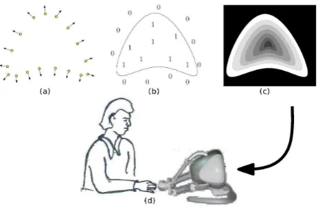
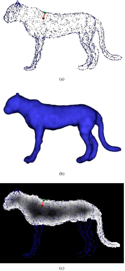
Visual rendering from point samples is a well studied problem in computer graphics. But a very little work has been done in the area of haptic rendering of a sparse point set data. Recon-struction from sparse data is an ill-posed problem and there is no unique solution. In surface reconstruction we are interested in finding a polygonal (commonly, a triangulated mesh) approx-imation of a moderately dense point cloud. In this paper we aim at finding a volumetric description of the object from an oriented sparse point set data suitable for haptic rendering. In order to ef-fectively render the object geometry, a 3D regular voxel grid is constructed and the minimum Euclidean distance of each grid node from the boundary of the object is calculated. We present a fast algorithm to compute the distance field specifically for a sparse data set. Once this distance field is calculated the object is haptically rendered using a proposed proxy based rendering method. The accuracy of the reaction force depend upon the ac-curacy with which the distance field is computed. Fig. 1a shows a scattered oriented point cloud in 2D for illustration. Our algo-rithm first compute a 3D indicator function (shown in Fig. 1a) from the scattered points and then computes the distance func-tion as shown in Fig. 1c. We propose a proxy based rendering of the computed distance function using a 3-DOF haptic device. To provide a combined hapto-visual immersion of the subject into the virtual world, the object is rendered visually using the zero iso-surface of the computed distance field. Sparse oriented

Fig. 1: Illustration of haptic rendering of distance field based description of an object from sparse oriented points.

point cloud data, in practice, may be generated using haptic scan-ning of a real non-deformable object. For haptic scanscan-ning of a given object, a force sensor may be attached to the haptic device to obtain the force along with the position information [10]. In the case of deformable objects there could be certain local de-formation of the object based on the Hooke’s law depending on the applied force by the haptic device. In that case an appropriate back projection is required to get the surface points.

The organization of the paper is as follows. An introduction to the relevant literature is given in section 2. Section 3 explains the proposed method of fast computation of distance field for sparse points, following which the rendering scheme is presented. The results of various experimentations are presented in section 4, and we conclude the paper in section 5.

2. LITERATURE REVIEW

function as the signed distance from the closest point of the es-timated tangent plane[9]. Level set based surface reconstruction method uses distance values accumulated in volumetric grid and the reconstructed surface is represented as the zero-isosurface of the scalar valued distance function[34]. There are also ap-proaches which combines global as well as local fitting scheme such as Poisson approximation by Hoppeet al.[12].

In the haptic rendering literature there are mainly two different approaches: Polygon based rendering and voxel based rendering. Some methods also use hybrid approaches[14]. A good introduc-tion to the basic haptic rendering technique is given by Salisbury et al.[28] and Laycocket al.[16]

2.1 Polygon Based Rendering

Traditional haptic rendering method is based on a geometric sur-face representation which consists of mainly triangular meshes. With polygon based rendering, each time when the haptic in-terface point (HIP) penetrates the object, the haptic rendering algorithm calculates the closest surface point on the polygonal mesh and the corresponding penetration depth. Ifxis the depth of penetration in the model, the reaction force can be calculated asF = ₋kx, wherekis the stiffness constant. Generally we assume the stiffness to be constant throughout the object. But it can be a function of position also, as is common for an ob-ject consisting of constituent materials with varying stiffness, ie,

k=K(x, y, z)where(x, y, z)are 3D coordinates. It is assumed thatK(x, y, z)is known.

The above method has problems while determining the appro-priate direction of the force while rendering thin objects. Zilles and Salisbury, and Ruspiniet al.independently introduced the concept of god-object[35] and proxy algorithm[26], respectively, which can solve the problems associated with thin objects. In the god-object rendering method, the authors use a second point in addition to the HIP called “god-object”, sometimes called the ideal haptic interface point (IHIP). While moving in free space the god-object and the HIP are collocated. But as the HIP pene-trates the virtual object, the god-object is constrained to lie on the surface of the virtual object. The position of the god-object can be determined by minimizing the energy of the spring between the god-object and the HIP, taking into account constraints rep-resented by the faces of the virtual object. If(x, y, z) are the coordinates of the virtual object and (xp, yp, zp) represents the coordinates of the HIP, the spring energy is given by

L=(x−xp)

2

2 +

(y₋yp)2 2 +

(z₋zp)2 2 +

l1(A1x+B1y+C1z−D1)+

l2(A2x+B2y+C2z−D2)+

l3(A3x+B3y+C3z−D3) (1)

whereLis the cost function to be minimized,l1,l2,l3 are

La-grange multipliers andA,B,C,Dare the homogeneous coef-ficients for the constraint plane equations. The ‘force shading’ technique (haptic equivalent of Phong shading) introduced by Morgenbesser and Srinivasan refined the above algorithm while rendering smooth objects[20]. One common problem with the mesh based representation is when the object is not fully en-closed by the bounding planes and a small hole may remain, where the IHIP sinks during the rendering process.

2.2 Voxel Based Rendering

The most basic representation for a volume is the classic voxel array in which each discrete spatial location has a one-bit label

indicating the presence or absence of material. Avilaet al.have used additional physical properties like stiffness, color and density during the voxel representation[3]. The voxmap-point shell algorithm uses the voxel map for stationary objects and point shell for dynamic objects[19][23]. Point shell has been defined as a set of point samples and associated inward facing normals. However, these normals are not available and one needs to compute the normal at every location.

The external surface∂Oof a solid objectOcan be described by the implicit equation[13] as

∂O=_{(x, y, z) _∈ R3

|φ(x, y, z) = 0_}

whereφis the implicit function (also called the potential func-tion) and(x, y, z)is the coordinate of a point in 3D. In other words the set of points for which potential is zero defines the implicit surface. This has found applications in haptic render-ing. Points with positive potential are outside the object and if

φ(x, y, z) <0then the point(x, y, z)is inside the surface. A volumetric surface can be defined as a discrete potential func-tion stored on a regular 3D grid. The potential at each point is a signed scalar value which indicates the proximity to the surface. Thus, in effect the potential function is nothing but the distance field of the point set defining an implicit surface. A distance field is a function where each point within the field represents the dis-tance from that point to the closest point on the bounding surface

∂Oand the sign denotes whether a given point is inside or out-side of a solid objectO. The usual convention is that the sign is negative for inside of the object[11].

The simplest way to compute the shortest distance to a set of sur-face points belonging to an object over a 3D discrete gridVis that, for each voxelv_∈Vthe distances to all the points are com-puted and the smallest one is stored. The 3D object geometry is commonly represented using triangular meshes. We can generate distance fields only from polygonal meshes which are closed. If

Nvis the number of voxels andNtis the number of triangles then the brute force method requiresNvNt steps to compute the distance field. For fast accessing of these triangles, hierar-chical data structures can be used. A basic approach to calculate distance to triangular patches has been explained by Payne and Toga[22]. Another hierarchical approach is the mesh sweeper al-gorithm proposed by Gu´eziec[8]. If the distance is needed only near the surface of the object, we can use a bounding volume around each triangle and can calculate the distances at grid nodes inside the specified bounding volume[7]. Mauch converted the features of a triangular mesh to a polyhedron[18], the feature, vertex becomes a cone with a polygonal base, edge becomes a wedge and the face becomes a prism. The polyhedron contain-ing points closer to the respective feature are then scan converted to compute the distances. Sigget al.used a graphic hardware to scan convert the characteristics for a faster implementation[30]. Once the distance close to the boundary is generated it may be propagated to the remaining volume. This is the principle of dis-tance transform. In Chamfer disdis-tance transform (CDT), the new distance of a voxel is computed from the distance of its neigh-bors by adding values from a distance template[25, 24]. In CDT the accuracy reduces as the distance from the surface increases. Similarly, a vector distance transform uses boundary conditions of voxels containing the vector to the closest point on the sur-face, and propagating these vectors according to a given vector template[21]. The fast marching method (FMM) technique was proposed first by Tsitsiklis[33] and then Sethian[29] which com-putes the arrival time of a front expanding in the normal direc-tion at a set of grid points by solving the Eikonal equadirec-tion from a given boundary condition.

dis-tances. Collision of the HIP with the objects and the correspond-ing penetration depth can be easily detected by computcorrespond-ing the potential at the HIP and hence an appropriate force can be ren-dered. However this rendering method also suffers from the thin object problem. So we propose a proxy based rendering on the computed distance field. For haptic rendering one should be able to render the object within 1msas any haptic interface system must be temporally sampled at a rate better than 1kHz[28]. In the next section we show how we can speed up the computation in case sparse point sets. For haptic rendering from dense point cloud data Leeperet.al.have proposed a locally computable im-plicit function method [17]. Instead of using a point proxy, a spherical volume proxy has been used in [31] and [27]. In the work by [32] rendering was restricted to a point cloud defined by Monge surface. The current work concentrate on how one can render sparse data set.

3. PROPOSED METHOD

The input data for our rendering technique is a set of sparse sam-pless(P,n)each consisting of a pointPand the corresponding outward facing unit normaln. We call this type of data as aug-mented point set. Note that the data(P,n)resembles more like the concept of a point shell defined in [23]. The proposed algo-rithm has two steps.

(1) distance field calculation from the augmented point set (P,n),

(2) haptic rendering with the computed distance field.

In order to find the bounding surface of the object represented by the sparse point set we initially find an indicator function (or characteristic function) from the given point set. The indicator function, in effect, divide the volume into two parts, inside and outside of the object bounding surface.i.e., the indicator function value is one for the region inside the object and zero outside. Once the indicator function is obtained the distance field can be found using technique explained in section sec. 3.2.

3.1 Computation of 3D Indicator Function

The volume reconstruction problem may be defined as: Given a sparse set of augmented points(P,n), find the bounding surface and hence the distance field over a uniform grid of voxels. We note here that we need to find the distance field for points ly-ing inside the objects only. Since there is no force field outside the object we need to search only in the direction opposite to the available outward surface normaln. For this, the following simple lemma is useful. The proof is quite easy and omitted.

LEMMA 1. When a single point and the direction of nor-mal at that point is given only one additional point is needed to uniquely define the sphere on which they both lie.

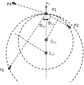
The bounding surface is obtained as a union of the minimum sized packing spheres for all points in the given data sets(P,n). This is illustrated for 2D case in Fig. 2. The pointP1andn1are

given. In order to mathematically find the embedded circle with the minimum radius, consider three pointsP2,P3 andP4 as

shown. We want to find the embedded circle of minimum radius atP1with at least one of these pointsP2,P3,P4on the circle.

Letaijbe the vector connecting pointitoj. If the dot product

−n1.a12is greater than zero (orθ12< π/2) it is possible to find

a circle withP2on its boundary. The radius of the corresponding

circle is given by

r12=

1

2|a12|sec(θ12), (2) from which we can calculate the center asc12=P1−r12.n1.

The pair(c12, r12)represents a unique circle withn1as the

out-ward normal atP1and both the pointsP1,P2on its

circumfer-ence. Similarly we can find another circle between the pointsP1

Fig. 2: Illustration of how to calculate the circle of minimum radius at a given sample point for a given point set.

Fig. 3: Illustration in 2D of (a) a sampled point set(P,n)for an arbitrary object, and (b) a packed circle (sphere in 3D) after mapping these points on a regular grid.

andP3of radiusr13=

1

2|a13|sec(θ13), whereθ13is the angle between the vectorsa13and−n1. Ifθij > π/2as with point P4, it is not possible to have a circle withP4 on the boundary.

Ifθij = π/2, it represents a circle with infinite radius. So we search only among the points withθ1j< π/2. At pointP1, we

find the minimum of all the radiirijfor all the sampled points

j= 2,3,4... This may be mathematically represented as

ri= min

j6=i rij ∀j (3)

whereriis the packing radius at the sample pointi. The min-imum of the calculated radius and its corresponding centerci represents the embedded circle atP1. Hence we observe that the

computation time for the embedding circle at every sample point is proportional to the number of sample points available. How-ever, one may further reduce the computation if only a smaller subset of points which are in the neighborhood ofP1is chosen

to reduce the search space. As mentioned earlier, the proposed method of computing the distance field is based on the concept of sphere embedding inside an object [4]. We start with forming a regular 3D grid of an appropriate resolution. The resolution could be dependent on how finely the object has been sampled and at what resolution it is required to be rendered in a given haptic platform. The algorithm is explained geometrically in 2D for better understanding.

Fig. 4: Illustration of how an improper sampling could introduce a large error in rendering the surface. The embedded circle ABC leaks out of the object as there is no sampled point near the corner P.

φ=d1

φ=d2

φ= 0

d2<0< d1 (xp, yp)

5φ(xp, yp)

(xh, yh)

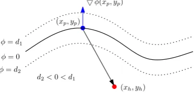
Fig. 5: Part of the distance function corresponding to an arbitrary object in 2D

such nodes and 0 for the remain nodes. If the sampled points are not dense enough, the embedded circle (sphere in the case of 3D) may leak out of the actual boundary of the object from which samples are taken. In Fig. 4 the rectangle is sampled sparsely and the sample points with normals are shown with arrows. In the figure we can see that near the densely sampled region most of the points inside the circles are inside the object. However, the circle ABC leaks out of the object by a large value as there are no points near the corner P.

3.2 Distance Field from Indicator Function

Distance field is computed only for the points inside the object. Using the method described in section 3.1 the 3D indicator func-tion is directly computed from the packed spheres. To find the distance field all the grid nodes with indicator function 0 are set as outside nodes. As we do not want to find the distance func-tion outside the object the outside nodes can be set with distance value 1. Now the grid nodes with at least one outside grid node in the nearest neighborhood is termed as boundary grid node. An iterative procedure is used to move the boundary node in-ward during the distance calculation. At each level of iteration the distance values are stored in the current boundary nodes are relabeled as outside node. In the initial level (level 0) we store the value zero as distance in the boundary nodes, next level (level 1) of boundary nodes with -1 level 2 with -2 and so on. This process is repeated until the total number of boundary nodes reduces to zero.

LetS be the set of all the inside nodes,δdenotes the boundary nodes. We use a structuring elementBof unit radius to erode the setS. Mathematically the distance field is computed as

φ(X) = 0 _∀ X_∈/S

= ₋n _∀ X_∈δ(S nB). (4)

3.3 Minimization of the Distance Between Proxy and HIP

Letφ(x, y, z)denotes the 3D potential function, then φ = 0 represents the zero iso-surface of the object which is actually the bounding surface of the object. In order to render the bounding surface of the object haptically we define a proxy which must not penetrate the bounding surface of the object but can move

freely over the surface. Our proxy based haptic rendering tech-nique minimizes the distance between proxy and HIP so that the proxy is constrained to move over the zero iso-surface of the object. To understand the minimization procedure consider an arbitrary 2D distance function shown in Fig. 5. There are three different contours shown in the figure corresponding to three dif-ferent iso values. The curve shown with thick blue line is the zero iso-contour of the object. The region above the zero iso-contour is outside the object boundary with distances greater than zero while the region below the zero iso-contour represents the inside region of the object with negative distances. The dotted line on either side of the zero iso-contour represents the iso-contour cor-responding to distancesd1 andd2whered1 <0 < d2. In the

figure proxy is shown with a blue circle and HIP with a red cir-cle.₅φ(xp, yp)shows the normal to the iso-contour at the proxy point. In free space the proxy position(xp, yp)should follow the HIP position(xh, yh). But when HIP is penetrated inside the ob-ject proxy moves over the obob-ject so as to minimize the distance between them. So we can write the objective function to be min-imized asψ(x, y, z)subject toφ(x, y, z) = 0where

ψ=(x−xh)

2

2 +

(y−yh)2 2 +

(z−zh)2

2 . (5)

We convert the constrained optimization problem as an uncon-strained one using the following objective function

Ψ =1

2|Xp−Xh|

2

+λ 2|φ(Xp)|

2

(6)

whereλis a regularization parameter. A gradient descent method can be used to minimize the cost functionΨ. Assuming the HIP to be fixed atXh, (ie, proxy updation is much faster than the haptic interaction which we show to be true in our experimental studies later)Ψcan be written as a function of current proxy positionXp only. So we can iteratively solve the problem by taking a small positive step sizeγ >0such that

X(k+1)

p =X

(k)

p −γ5Ψ(X

(k)

p ) (7)

whereX(pk)and5Ψ(X

(k)

p )are the proxy location and the gradi-ent of the objective function, respectively, in the currgradi-ent iteration andX(pk+1)is the proxy location for the next iteration. The gra-dient of the objective function can be computed as

5Ψ(X(k)

p ) = (Xp−Xh)(k)+λφ(X(pk))5φ(X

(k)

p ). (8) Substituting equation (8) in equation (7), the resulting solution becomes

X(k+1)

p =X

(k)

p −γ(Xp−Xh)(k)−βφ(X(pk))5φ(X

(k)

p ) (9)

where the constantβ=γλ,(Xp−Xh)is the vector from HIP to the proxy and₅φ(X(pk))is the gradient of the distance function at the current proxy location. In the solution given in equation (9), the term(Xp−Xh)tries to minimize the distance between HIP and proxy while the termφ(Xp)5φ(Xp)keeps the proxy near the bounding surface of the object during collision. When

φ(Xp)<0, proxy is outside the object and the resulting solution becomesXp=Xh.

3.4 Haptic Rendering

As the distance samples are stored on a regular grid, distance at any point inside the grid can be interpolated from the 8 nearest neighboring grid nodes. The gradient can also be computed at all the nodes directly from the distance field. Haptic rendering process includes two steps.

3.4.1 Collision between the HIP and the object:. As we move the haptic device inside the 3D grid the distance is computed at the proxy location,Xpby trilinear interpolation of the distance stored at the grid location. If the interpolated distance is greater than zero, the proxy lies outside the object, proxy moves with the HIP, no collision is detected and therefore no force is fed back.

3.4.2 Force Computation for Rendering:. If the interpolated distance at the proxy location is less than zero a collision is de-tected and an appropriate force has to be fed back. Once colli-sion is detected proxy moves tangentially over the iso-surface so as to minimize the distance between proxy and HIP as discussed in sec. 3.3, while the reaction force is as given in equation (10) wherekis the Hooke‘s constant andXh−Xpis the penetration depth of HIP in the object.

f=₋k(Xh−Xp). (10)

4. EXPERIMENTAL RESULTS

The proposed method was implemented in visual C++ in a win-dows XP platform with a CORE 2QUAD CPU @ 2.66GHZ with 2GB RAM. In order to generate the data set for our algorithm, we created virtual objects using polygonal meshes and they are rendered haptically with the standard god-object rendering tech-nique. These virtual objects are scanned manually using a 3-DOF haptic device and the position and force values are sampled at different points. The distance field is calculated in a fixed regu-lar grid of size 300X300X300. The size and spatial resolution of the grid depend on two factors: the interaction space of the haptic device used to render the object and the resolution at which the object should be rendered. We use a 3-DOF haptic device from NOVINT with a 4 inch cube haptic interaction space. Moreover, the object is visually rendered as points on the zero-iso-surface of the computed distance field. This allows the user a joint hapto-visual experience while touching the object. We have selected the above grid size with an appropriate resolution so as to fit the active space of the haptic device suitable with our experimental setup. During the haptic rendering phase, the calculation of force at a point takes only 0.02mswith the above grid size, which is much lower than the required limit of 1msfor a smooth haptic rendering.

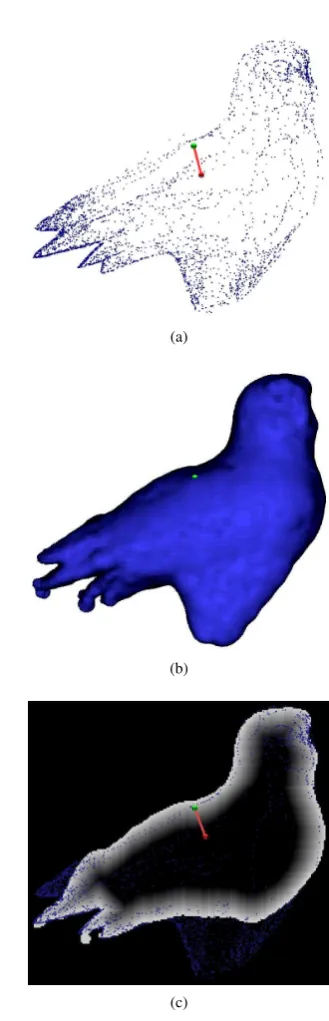
Depending on the size and shape of the object the distance field computation may use only a small portion of the grid size. For example, the point cloud data shown in Fig. 6 with 3,725 points uses a grid of size 186X173X87 and it took approximately 38.09 seconds to calculate the precomputable distance field. The algo-rithm computes the distance values at 8,24,463 inside grid nodes. The zero iso-surface are shown in Fig. 6(b) for the visual render-ing purpose. The green sphere in the figure shows the proxy point and the red sphere shows the HIP point during the rendering pro-cess. The red line indicate the penetration depth at the shown HIP point. The user experience on handling the object in the haptic space was also found to be very satisfactory.

Another sparse oriented point cloud data shown in Fig. 8a has 5153 points. The distance field is computed in a grid of size 126X187X72. The computation time is 26.25sfor 3,04,072 in-ternal nodes. The proxy and HIP positions are also shown in the figure. Point set data with 3751 points are shown in Fig. 8b. It took 110.82 seconds to calculate the distance field at 11,29,209 inside points. Another point set data corresponding to a water hy-drant is shown in Fig. 8c with 3756 points. Distance field is com-puted at 5,86,222 points in 30.86 seconds. Augmented point set datas(P,n)is generated by haptic scanning of a given polygo-nal mesh using a 3-DOF haptic device. To perform haptic sam-pling the polygonal mesh is haptically rendered using the god object rendering technique. The position of the haptic device and the corresponding reaction force are sampled during the interac-tion with the object. The device posiinterac-tions corresponding to the non zero force sample are then projected back to the surface to

(a)

(b)

(c)

Fig. 6: (a) Scattered oriented points and (b) zero iso-surface of the dis-tance field visually rendered using a known light source direction (c) distance field for a particular cross section of the object (data courtesy: ‘www.top3dmodels.com’).

get the point set, the direction of reaction force gives the orien-tation of each point.

In practice it is not required to find the distance field at all the inside grid nodes, since the proxy rarely sinks more than 3-4 voxel length in the object during the minimization of equation (6). Distance calculation only up to 5 or 6 nodes inside the actual bounding surface nodes is enough for a stable haptic feedback. Table. 1 compares the computational time requirement for differ-ent data sets. Note that this is required to be pre-computed only once following while the haptic interaction could be very fast as the proxy updation requires 0.02ms only.

(a)

(b)

(c)

Fig. 7: (a) Scattered oriented points and (b) zero iso-surface of the dis-tance field visually rendered using a known light source direction (c) distance field for a particular cross section of the object (data courtesy: ‘www.turbosquid.com’).

Table 1. : Summary of computational requirement for various point cloud data used.

Object Number of Number of Distance field name oriented inside computation points nodes time (s)

Hydrant 3,756 5,86,222 30.86

Owl 3,725 8,24,436 38.09

Boy 5,153 3,04,072 26.26

Bomberman 3,751 11,29,209 110.82

Jaguar 4,433 1,34,987 11.673

(a)

(b)

(c)

Fig. 8: Scattered oriented points, visually rendered zero iso-surface of the distance field for a known light source direction and a cross section of the computed distance field for 3 different objects. (a) boy (b) bomberman (c) water hydrant (data courtesy: ‘www.turbosquid.com’).

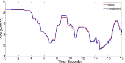
known spherical object such that the bounding surfaceφ(X)is precisely known. The rendered reaction force for a particular in-teraction with the object is compared with the force computed using the known, implicit equation of the sphere. The reason for selecting a sphere for the comparison purpose is that the sphere equation can readily give the penetration depth of the HIP in the object. The surface of the sphere is interacted with a 3-DOF hap-tic device. The haphap-tic position and the corresponding rendered reaction force are sampled from the device during the interaction. The ideal reaction force is computed using the implicit sphere equation. The magnitude of force is plotted as a function of time for both the cases and is shown in Fig. 9. The red line in the figure shows the force computed using the implicit sphere equa-tion. The blue line shows the rendered force using the proposed technique. The rendered force can be seen to be very close to the actual force substantiating our claim that the proposed method does provide a good haptic experience to the user.

5. CONCLUSIONS

Fig. 9: Comparison of the rendered force with the ideal one for a partic-ular interaction with a known spherical object.

cloud in a regular 3D grid of voxels. Once the points are mapped to the nearest nodes, all the remaining processing is done only in the 3D grid. Distance field is sampled in each grid node by the method of embedded spheres inside the object. The zero-isosurface of the distance field which is the boundary surface of the object is visually shown for a combined hapto-visual experi-ence. In effect we use a distance field based haptic rendering and a simultaneous point based graphic rendering. We validated our results using scattered oriented data corresponding to a spherical object and found that the proposed rendering method works very well with scattered data.

6. REFERENCES

[1] Nina Amenta, Marshall Bern, and Manolis Kamvysselis. A new Voronoi-based surface reconstruction algorithm. In SIGGRAPH, pages 415–421, 1998.

[2] Nina Amenta, Sunghee Choi, and Ravi Krishna Kolluri. The power crust, unions of balls, and the medial axis trans-form.Computational Geometry: Theory and Applications, 19:127–153, 2000.

[3] Ricardo S. Avila and Lisa M. Sobierajski. A haptic inter-action method for volume visualization.Visualization Con-ference, IEEE, 0:197, 1996.

[4] Ilya Baran and Jovan Popovic. Automatic rigging and an-imation of 3d characters. ACM Trans. Graph., 26(3):72, 2007.

[5] Fausto Bernardini, Joshua Mittleman, Holly Rushmeier, Claudio Silva, Gabriel Taubin, and Senior Member. The ball-pivoting algorithm for surface reconstruction. IEEE Transactions on Visualization and Computer Graphics, 5:349–359, 1999.

[6] J. C. Carr, R. K. Beatson, J. B. Cherrie, T. J. Mitchell, W. R. Fright, B. C. McCallum, and T. R. Evans. Reconstruction and representation of 3D objects with radial basis func-tions. InComputer Graphics (SIGGRAPH 01 Conf. Proc.), pages 6776. ACM SIGGRAPH, pages 67–76. Springer, 2001.

[7] Frank Dachille and Arie Kaufman. Incremental triangle voxelization. InGraphics Interface, pages 205–212, 2000. [8] Andr´e Gu´eziec. ’Meshsweeper’: Dynamic Point-to-Polygonal-Mesh Distance and Applications. IEEE Transactions on Visualization and Computer Graphics, 7:47–61, January 2001.

[9] Hugues Hoppe, Tony DeRose, Tom Duchamp, John Mc-Donald, and Werner Stuetzle. Surface reconstruction from unorganized points. In COMPUTER GRAPHICS (SIG-GRAPH 92 PROCEEDINGS), pages 71–78, 1992. [10] R. Hover, M. Harders, and G. Szekely. Data-driven

hap-tic rendering of visco-elashap-tic effects. InProceedings of the

2008 Symposium on Haptic Interfaces for Virtual Environ-ment and Teleoperator Systems, pages 201–208, Washing-ton, DC, USA, 2008. IEEE Computer Society.

[11] Mark W. Jones, J. Andreas Brentzen, and Milos Sramek. 3D Distance Fields: A Survey of Techniques and Appli-cations.IEEE Transactions on visualization and Computer Graphics, 12(4):581–599, 2006.

[12] Michael Kazhdan, Matthew Bolitho, and Hugues Hoppe. Poisson surface reconstruction. In Proceedings of the fourth Eurographics symposium on Geometry processing, SGP ’06, pages 61–70, Aire-la-Ville, Switzerland, Switzer-land, 2006. Eurographics Association.

[13] Laehyun Kim, Anna Kyrikou, Mathieu Desbrun, and Gau-rav Sukhatme. An implicit-based haptic rendering tech-nique. InProceeedings of the IEEE/RSJ International Con-ference on Intelligent Robots, volume 3, pages 2942–2948, 2002.

[14] Laehyun Kim, Gaurav S. Sukhatme, and Mathieu Desbrun. A haptic rendering technique based on hybrid surface rep-resentation. IEEE Computer Graphics and Applications, Special Issue on Haptic Rendering - Beyond Visual Com-puting, 24(2):66–75, March 2004.

[15] Ravikrishna Kolluri, Jonathan Richard Shewchuk, and James F. O’Brien. Spectral surface reconstruction from noisy point clouds. InProceedings of the 2004 Eurograph-ics/ACM SIGGRAPH symposium on Geometry processing, SGP ’04, pages 11–21, New York, NY, USA, 2004. ACM. [16] S. D. Laycock and A. M. Day. A survey of haptic

render-ing techniques.Computer Graphics Forum, 26(1):50–65, March 2007.

[17] Adam Leeper, Sonny Chan, and Kenneth Salisbury. Con-straint based 3-DOF haptic rendering of arbitrary point cloud data. InRSS Workshop on RGB-D Cameras, Univer-sity of Southern California, June 2011.

[18] Sean Mauch. A fast algorithm for computing the closest point and distance transform. Technical report, California Institute of Technology, 2000.

[19] William A. Mcneely, Kevin D. Puterbaugh, and James J. Troy. Six degree-of-freedom haptic rendering using voxel sampling. InProc. of ACM SIGGRAPH, pages 401–408, 1999.

[20] Srinivasan M. A. Morgenbesser, H.B. Force shading for haptic shade perception. InProceedings of the ASME Dy-namic Systems and Control Division, volume 58, pages 407–412, 1996.

[21] James C. Mullikin. The vector distance transform in two and three dimensions.CVGIP: Graph. Models and Image Process., 54:526–535, November 1992.

[22] Bradley A. Payne and Arthur W. Toga. Distance field ma-nipulation of surface models.IEEE Comput. Graph. Appl., 12:65–71, January 1992.

[23] Matthias Renz, Carsten Preusche, Marco Ptke, Hans peter Kriegel, and Gerd Hirzinger. Stable haptic interaction with virtual environments using an adapted voxmap-pointshell algorithm. InProc. Eurohaptics, pages 149–154, 2001. [24] Frank Rhodes. Discrete Euclidean metrics.Pattern Recogn.

Lett., 13:623–628, September 1992.

[25] Azriel Rosenfeld and John L. Pfaltz. Sequential operations in digital picture processing.J. ACM, 13:471–494, October 1966.

[26] Diego C. Ruspini, Krasimir Kolarov, and Oussama Khatib. The haptic display of complex graphical environments. In Proc. of ACM SIGGRAPH, pages 345–352, 1997. [27] Fredrik Ryden, Sina Nia Kosari, and Howard Jay Chizeck.

[28] Kenneth Salisbury, Francois Conti, and Federico Barbagli. Haptic rendering: Introductory concepts.IEEE Computer Graphics and Applications, 24(2):24–32, 2004.

[29] J A Sethian. A fast marching level set method for mono-tonically advancing fronts. Proceedings of the National Academy of Sciences of the United States of America, 93(4):1591–1595, 1996.

[30] Christian Sigg, Ronald Peikert, and Markus Gross. Signed distance transform using graphics hardware. In Proceed-ings of the 14th IEEE Visualization 2003 (VIS’03), VIS ’03, pages 83–90, Washington, DC, USA, 2003. IEEE Com-puter Society.

[31] K. G. Sreeni and Subhasis Chaudhuri. Haptic Rendering of Dense 3D Point Cloud Data. InIEEE Haptic Symposium, pages 333–339, Vancouver, BC, Canada, March 4-7 2012. [32] K. G. Sreeni, K. Priyadarshini, A. K. Praseedha, and

Sub-hasis Chaudhuri. Haptic Rendering of Cultural Heritage

Objects at Different Scales. InEurohaptics, Tampere, Fin-land, June 12-15 2012.

[33] John N. Tsitsiklis. Efficient algorithms for globally opti-mal trajectories.IEEE Transactions on Automatic Control, 40(9):1528–1538, 1995.

[34] Hong-Kai Zhao, Stanley Osher, and Ronald Fedkiw. Fast surface reconstruction using the level set method. In Pro-ceedings of the IEEE Workshop on Variational and Level Set Methods (VLSM’01), VLSM ’01, pages 194–, Wash-ington, DC, USA, 2001. IEEE Computer Society.