Munich Personal RePEc Archive
An Estimation of Residential Water
Demand Using Co-Integration and Error
Correction Techniques
Martinez-Espineira, Roberto
April 2005
Online at
https://mpra.ub.uni-muenchen.de/615/
An Estimation of Residential Water Demand Using Co-Integration
and Error Correction Techniques
Abstract
In this paper short- and long-run price elasticities of residential water demand are estimated using co-integration and error-correction methods. Unit root tests reveal that water use series and series of other variables affecting use are non-stationary. However, a long-run co-integrating relationship is found in the water demand model, which makes it possible to obtain a partial correction term and to estimate an error correction model. The empirical application uses monthly time-series observations from Seville (Spain). The price-elasticity of demand is estimated as around -0.1 in the short run and -0.5 in the long run. These results are robust to the use of different specifications.
JEL Classification: C22, D12, Q25.
Keywords: seasonal unit roots, residential water demand, price elasticity, time-series, co-integration, Error Correction Model.
Introduction
While it is generally agreed that residential water users’ short-run and long-run reactions
to price changes might be substantially different, long-run water demand elasticities have
been rarely estimated for European users. The main purpose of this paper is to estimate
and compare short-run and long-run price elasticities of residential water demand using
data from Seville (Spain). A secondary objective is to assess the usefulness of the
tech-niques of co-integration (see Engle and Granger, 1987; Johansen, 1988, among others)
and error correction (Hendry, Pagan, and Sargan, 1984) in the analysis of these
price-elasticities of water demand. To the author’s knowledge, no previous published work has
applied this econometric methodology to the study of water demand, while it has proved
very useful to estimate the demand for other types of transformed natural resources, such
as gasoline and electricity. The analysis in this paper is similar to these previous studies
in that it deals with a resource whose price could affect purchase patterns of capital stock
(water-using appliances) and whose consumption might respond partly to habit.
Monthly time-series data on price and aggregate residential consumption over a
ten-year period are matched with climatic data, data on non-price demand policies, and
av-erage income. The availability of monthly data allows not only for the use of much more
accurate measures of consumption but also to test for seasonal effects in consumption
and the peculiarities of dynamic effects that cannot be captured when using yearly data.
The city of Seville was chosen as a case study because it has been already the subject of
several analyses based on a variety of econometric specifications. This makes it possible
to compare the results of the present study with alternative ones.
The econometric estimation proceeds in two steps. First, unit root tests are conducted
relationship between price and consumption is estimated. The stationarity of the different
time-series involved is investigated using seasonal unit root tests and tests that consider
structural breaks in the series . The long-run equilibrium relationship is then used as an
error correction term in an error correction model (ECM henceforth). These techniques
provide measures of the short- and long-run elasticities as well as the speed of adjustment
towards long-run values. The elasticities estimated suggest, as it has been found in the
literature, that household water demand is inelastic with respect to its own price but not
perfectly so. The results show remarkable consistency between the different techniques
used to analyze the dynamics of the relationships.
This paper is organized as follows. Section 1 lists some previous studies dealing with
the estimation of residential water demand and applied works that use the techniques
of co-integration and error correction. The characteristics of water demand in Seville are
described in Section 2 and the data set is described in Section 3. The econometric methods
and the results are presented in Sections 4 and 5 respectively. Section 6 concludes.
1
Background
Residential water demand has been extensively analyzed during the last decades. The
main objective of this research is to estimate price elasticities of water demand from
wa-ter demand functions where either individual or aggregate residential wawa-ter use is made
dependent on water price and other variables such as income, climatic conditions and
type of residence. Water demand appears as inelastic but not perfectly inelastic. Most
applied studies focus on areas of the USA (e.g. Schefter and David, 1985; Chicoine
and Ramamurthy, 1986; Nieswiadomy and Molina, 1989; Renwick and Green, 2000).
and Thomas (2000), and Martínez-Espiñeira (2002). Due to differences in the way water
is used and the way in which it is priced, there are sharp geographic variations in the
size of price elasticities of water demand, especially between Europe and North America
(Arbués et al., 2003; Dalhuisen et al., 2003). Therefore, it is important that European
policy makers be provided with the results from analyses based on European data that
consider long-run versus short-run usage responses to price changes.
A number of previous studies have found short-run elasticities smaller than their
long-run counterparts. This suggests that consumers might need time to adjust their
water-using capital stock and to learn about the effects of their use on their bills. These studies
use some type of flow-adjustment model, where lagged consumption is included as an
explanatory variable. The latter assumes that the actual adjustment to consumption is a
fixed ratio of the totaldesired or equilibrium adjustment. The short-run elasticity is then
given by a choice of utilization rate of the water-using capital stock, while the long-run is
defined as the choice of both the size of this capital stock and the intensity of its use. Past
consumption is introduced in the model with lags of different length and shape. Agthe et
al. (1986), Moncur (1987), Lyman (1992), Dandy et al. (1997) are examples of this type of
approach, while somewhat more sophisticated econometric techniques have recently been
applied, including the use of dynamic panel data methods (Nauges and Thomas, 2001).
Lack of data on water-using capital stock usually prevents the use of stock-adjustment
models, although in some cases (Agthe et al., 1986) a time variable proxies the evolution
of the capital stock. Renwick and Archibald (1998) introduce information available on
water related technology in a model that explicitly analyzes endogenous technical change.
These studies find that, in agreement with economic theory, short-run responses to price
changes are weaker than long-run ones. However, Agthe and Billings (1980) find, using a
long-run value (-0.672), suggesting that, with monthly data, there could be a short-run
overreaction to price changes and that alternative techniques of time-series analysis might
help solve these inconsistencies.
None of these studies has used co-integration and/or error correction techniques to
estimate short-run and long-run price effects. These methods have been extensively used
since Engle and Granger’s 1987 seminal paper. Electricity demand forecasting is among
the earliest applications of co-integration (Engle et al., 1989). More recently, co-integration
and error correction have been applied to the estimation of energy and gasoline demand.
For example, Bentzen (1994), Eltony and Al-Mutairi (1995), and Ramanathan (1999)
study the behavior of gasoline consumption. Fouquet (1995) investigates the impact of
VAT introduction on residential fuel (coal, petrol, gas, and electricity) demand in the
United Kingdom, while Beenstock et al. (1999) address the issue of seasonality in electricity
consumption. Using co-integration analysis to estimate demand functions avoids problems
of spurious relationships that bias the results and provides a convenient and rigorous way
to discern between short-run and long-run effects of pricing policies.
2
Water demand in Seville
Residential water use represents about 74% of the demand for drinking water in the Seville
and its metropolitan area. This proportion remained fairly constant during the nineties,
except in 1992-93, when the Universal Exposition increased the share of institutional use
(EMASESA, 2000, pp. 2-3). The total number of families living in the city of Seville in 1998
was 226,692 and the water supplier,EMASESA, had a total of 190,759 domestic customers
at the end of 1998. The number of customers has increased significantly since 1997. This
collective meters by individual meters, causing an increase in the average yearly growth
of the number of domestic customers from 7% to %10-11 (EMASESA, 2000, p. 4).
According to company’s estimates, Sevillan households use 53% of the water in the
toilet, in the kitchen, and for washing clothes. These components could be significantly
affected by the efficiency of water-using equipment and the frequency of its renewal. An
extra 39% is used in showers, which could be determined by both habits and the
charac-teristics of water-use equipment. Outdoor use is minimal (EMASESA, 2000, p. 7).
Seville suffered a serious draught between 1992 and 1995, during which important
savings were achieved through measures such as media campaigns, municipal edicts and the
ban of certain uses, water restrictions, and consumption control inspections. At the height
of the drought, savings of around 25% with respect to previous years were achieved. In
mid-1992, imbalances between supply and demand started to arise. Media campaigns were
launched to ask for voluntary water conservation. Then this was made compulsory, since
from September water supply was reduced to 20 hours daily, inducing savings of 15%. Daily
water supply was reduced to 16 hours and at the end of 1992 consumption began to reflect
a 25% reduction. At the beginning of 1993 the company had to resort to the emergency
intakes as the only source of supply. During the first half of 1995, a 28% reduction with
respect to the consumption previous to the drought was achieved. Restrictions increased to
10 hours a day. Eventually, the rain came at the end of 1995 and the drought was overcome
thanks to the savings achieved in that period. The awareness campaign continued (in
spite of the reservoirs having enough water) to maintain the population’s saving habits
(EMASESA, 2000, pp. 6-7). A more detailed description of the measures implemented to
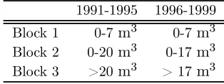
Table 1: Evolution of pricing-block sizes.
1991-1995 1996-1999 Block 1 0-7m3 0-7m3
Block 2 0-20m3 0-17 m3
Block 3 >20m3 > 17m3
3
Dataset description
EMASESA, the private company in charge of supplying water and sewage collection
ser-vices in Seville provided the main data used for the estimations. They include information
for the period 1991-1999 on tariffs, number of domestic accounts, and total domestic use.
The tariffconsists of afixed quota and an increasing three-block rate. Table 1 shows
the evolution of the block sizes. The price for the first seven-unit block applies only to
those users who use a total of less than seven cubic meters. If the consumer exceeds this
level of use, the price of the second block applies also to thesefirst seven cubic meters. This
type of step-rate structure is in this case explicitly aimed at rewarding water conservation
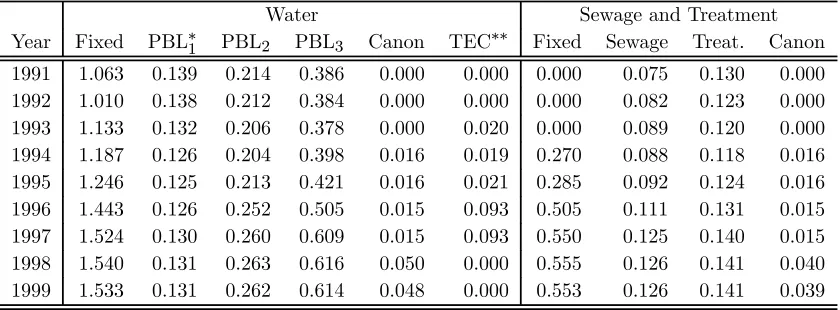
efforts. The rest of the tariffis based on conventional increasing blocks. The tariffincludes
a water supply fee, a sewage collection fee, and a treatment fee, and, from 1994, a
waste-water infrastructure fee (canon) was collected on behalf of the Andalusian government.
Finally, from 1993 to 1997, a temporary extra fee was charged for the company’s finances
to recover from the impact of the drought. The value of the fixed quota depends on the
size of the meter, but the most common one for domestic users (13 mm) was adopted. The
evolution of the prices in each block between 1991 and 1999, including all the elements
of the water and sewage bill, is detailed in Table 2. All prices are expressed in constant
pesetas (ESP) of 1992, translated into EURO equivalents (1 EURO = 166.386 ESP).
Table 2: Tariffevolution (1992 EURO equivalents, excluding VAT).
Water Sewage and Treatment Year Fixed PBL∗
1 PBL2 PBL3 Canon TEC∗∗ Fixed Sewage Treat. Canon
1991 1.063 0.139 0.214 0.386 0.000 0.000 0.000 0.075 0.130 0.000 1992 1.010 0.138 0.212 0.384 0.000 0.000 0.000 0.082 0.123 0.000 1993 1.133 0.132 0.206 0.378 0.000 0.020 0.000 0.089 0.120 0.000 1994 1.187 0.126 0.204 0.398 0.016 0.019 0.270 0.088 0.118 0.016 1995 1.246 0.125 0.213 0.421 0.016 0.021 0.285 0.092 0.124 0.016 1996 1.443 0.126 0.252 0.505 0.015 0.093 0.505 0.111 0.131 0.015 1997 1.524 0.130 0.260 0.609 0.015 0.093 0.550 0.125 0.140 0.015 1998 1.540 0.131 0.263 0.616 0.050 0.000 0.555 0.126 0.141 0.040 1999 1.533 0.131 0.262 0.614 0.048 0.000 0.553 0.126 0.141 0.039 * PBLi = water price in block i.
**TEC = Temporary Extra Charge
trefers to Montht):
• Qt (m3/capita month) is average per capita domestic water use. The raw data
con-sist of 108monthly values for total use. The company reads meters continuously at
quarterly intervals for each individual meter and estimates monthly use in the
follow-ing manner. For each individual, the average daily use durfollow-ing the readfollow-ing period is
calculated, then this average use is allocated to each month according to the number
of days corresponding to that month in that particular reading period.1 Although
this procedure smooths off all intermonthly variation at the individual level, the
estimated aggregate use mimics the actual pattern of intermonthly variation, since
there is a large number of individual meters and they are read continuously. Annual
data on the number of accounts were also collected. However, instead of using this
variable to calculate average water use per account, values of total population in
1For example, if the reading period goes from 28-04-00 to 03-08-00 and the reading is 91 m3
, since the length of the period is 97 days, average daily use is 0.93 m3
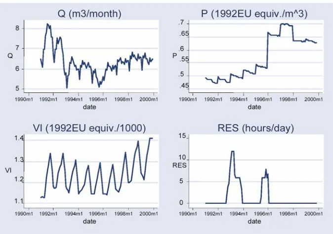
Figure 1: Evolution of the water use (Q), water marginal price (P), virtual income (V I)
and water restrictions (RES) variables.
Seville were used to calculate monthly average use per capita. The reason is that
during the study period the water company substantially increased the number of
individual meters. The evolution of the values of both consumption per account and
inhabitants per account strikingly show this effect of the introduction of individual
meters described in Section 2. Figure 1 shows the evolution of the values of Qt,
including the effect of the drought during the first half of the decade. Conservation
efforts persisted after the end of the drought, as described in Section 2, and water
use levels did not fully return to pre-drought levels
• Pt (1992 EURO equivalents/m3) is the marginal price of water. It corresponds to
a variation on the Taylor-Nordin specification (Taylor, 1975; Nordin, 1976) for
and difference are derived from an artificial linearization of the tariff structure by
regressing the constructed bill amounts associated with each integer value of
poten-tial (between 1 m3 and 25 m3) monthly water use per account on these water use
values. This instrumental marginal price is the slope of that estimated regression.
The estimated intercept provides an estimate for the Taylor-Nordin difference. This
price formulation avoids problems of price endogeneity and reflects the fact that
con-sumers have only an imperfect knowledge of the tariffstructure and the block they
are consuming in at each point in time. The strict application of the Nordin-Taylor’s
original specification has been the subject of debate (discussed in Arbués et al. ,
2003). A perfectly informed consumer would react to the marginal price and the
rate premium, but most consumers will not carefully study the tariff structure or
changes in inframarginal rates because of information costs. Alternative approaches
include the use of the average price, or both average and marginal price in the
same or different models. The modified Nordin-Taylor specification was chosen for
this study in light of the results obtained with different specifications by
Martínez-Espiñeira (2002) in other Spanish regions and because it was successfully applied
by Martínez-Espiñeira and Nauges (2004) in a previous study in Seville, which also
makes it possible to compare results based on the same price specification but
dif-ferent econometric models. Additionally, the recent analysis by Taylor et al. (2004)
casts doubts on the alleged empirical superiority of the average price specification.
Monetary values were deflated using the official provincial-wise retail price index.
No single available series of the price-index would be long enough to cover the whole
price series, so the published series with base 1983 was adapted to merge with the
• V It (1992 EURO equivalents) is virtual income. It is the difference between the
average salaries (Wt) and Dt, the instrument for the Nordin-difference (Nordin,
1976) variable. It is the intercept of the estimated linear function used to derive P
and it can be included as part of the virtual income definition, since it only exerts
an income effect caused by the nonlinearity of the tariffstructure (Billings, 1982),
so, theoretically, its coefficient would have the same magnitude and opposite sign
as the one of income.2 The average salaries series (from the Instituto Nacional de
Estadística) is used to proxy for household income. It had originally a quarterly
frequency, so it was linearly interpolated to get monthly values. The values for
Pt and Dt were calculated using the tariff schedules applied in each period. The
evolution of this series is shown in Figure 1
• RAINtis the current level of precipitation. Unit: mm/month.
• T EM Ptis the average of the daily maximum temperatures in Montht. Unit: ◦C/10
• RESt(hours/day) refers to the number of daily hours of supply restrictions applied
as part of the emergency control measures during the worst drought periods. The
number of hours of restriction a day is weighted by the number of days in the month
to which that number applied. This variable has been calculated directly from the
relevant city council drought-emergency decrees (EMASESA, 1997).The evolution of
this series is shown in Figure 1
• BANt is a binary variable with value 1 when temporary outdoor-use bans were
applied during the drought.
2By lumpingDtogether with income the theoretical prediction is imposed as a restriction. In practice
the effect of this variable on its own would not be significant, since the water bill amounts to such a small
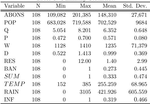
Table 3: Summary Statistics.
Variable N Min Max Mean Std. Dev. ABONS 108 109,082 201,385 148,310 27,671 POP 108 683,028 719,588 702,529 9684 Q 108 5.054 8.201 6.352 0.648 P 108 0.472 0.700 0.571 0.080 W 108 1128 1410 1235 71,379 D 108 0.522 1.413 0.999 0.369 RES 108 0 12.00 1.40 2.99 BAN 108 0 1 0.273 0.445
SU M 108 0 1 0.333 0.474
T EM P 108 152 385 255.259 68.965 RAIN 108 0 3105 421.926 605.559 INF 108 0 1 0.319 0.466
• IN Ft is a binary variable with value 1 if water conservation information campaigns
were being applied during the drought
• SU Mt is a binary variable with value 1 in May, June, July, and August
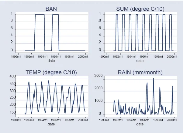
The evolution of the BAN, SU M, T EM P and RAIN series is shown in Figure 2.
Summary statistics for all variables are provided in Table 3. Evolution of the outdoor-use
bans (BAN), summer dummy (SU M), average maximum daily temperatures (T EM P)
and monthly precipitation (RAIN) variables.
4
Econometric methods
The techniques of co-integration (see Engle and Granger, 1987) and error correction (see
Hendry et al., 1984, among others) are used to investigate the dynamics of household
water consumption and to measure the short-run and long-run effects of the price of water
Figure 2: Evolution of the outdoor-use bans (BAN), summer dummy (SU M), average
maximum daily temperatures (T EM P) and monthly precipitaion (RAIN) variables.
Let us consider the simple form of a dynamic model:
yt=µ+γ1yt−1+β0xt+β1xt−1+εt, t= 1, . . . , T, (1)
where yt and xt could represent respectively consumption and price at time t. The error
term (εt) is assumed independently and identically distributed. We will assume in the
following that xt is a one-dimensional vector for ease of exposition. µ,γ1,β0,β1 are
un-known parameters. In Model 1 the short-run and long-run effects ofx ony are measured
respectively byβ0 and(β0+β1)/(1−γ1). Re-arranging terms, we obtain the usualECM:
∆yt=µ+β0∆xt−(1−γ1)(yt−1−θxt−1) +εt, t= 1, . . . , T, (2)
Thus, the estimation of theECM gives directly a measure of the short-run and long-run
effects ofxonythrough the estimates ofβ0andθ. The term (yt−1−θxt−1) in Model 2 can
be seen as apartial correction for the extent to whichyt−1 deviated from the equilibrium
value corresponding toxt−1. That is, this representation assumes that any short-run shock
toythat pushes it offthe long-run equilibrium growth rate will gradually be corrected, and
an equilibrium rate will be restored. The expression (yt−1−θxt−1) is theresidual of the
long-run equilibrium relationship betweenx andy.3 Therefore, this error correction term
will be included in the model if there exists a long-run equilibrium relationship between
x and y or, in other words, if both series are co-integrated in the sense of Granger (see
Engle and Granger, 1987). If the series are co-integrated they will, in the long run, tend to
grow at similar rates, because their data generating processes may be following the same
stochastic trend, or may share an underlying common factor.
For any0<γ1<1, the absolute value ofθwill exceed the absolute value of β0 as long
as β0 and β1 have the same sign. Under such likely conditions, the long-run adjustment
to a change in the price of water will be weaker than the short-run adjustment. Although
it would be a rare occurrence in practice, households might instead overreact in the short
run to changes in prices. This effect has been observed in applications focusing on other
commodities (Fouquet, 1995).
The econometric analysis will proceed in two steps. In the first step, we test if x
and y are co-integrated series, by testing for the stationarity of the series. If the series
are integrated of the same order, a co-integrating vector might be then found such that
a linear combination of the non-stationary variables obtained with that vector is itself
stationary. If this proves to be the case, the estimation of the Granger co-integration
3For this reason, it is commonly said that (1
−γ1) provides a measure of thespeed of adjustmenttowards
relationship will give a measure of the long-run effect of x on y. In a second step, the
co-integration residuals are used as an error correction term in the ECM above and the
short-run effect and the speed of adjustment can be estimated.
4.1
Tests for order of integration
A time series is I(i) (integrated of order i) if it becomes stationary after differencing it
i-times. A non-stationary series can be represented by an autoregressive process of order
p, so unit-root tests for a variableytusually rely on transformed equations of the form:
∆yt=µ+λt+ (γ−1)yt−1+
p−1
X
i=1
γj∆yt−i+εt (3)
This test, known as the Augmented Dickey Fuller,ADF, (Dickey and Fuller, 1981) allows
for anAR(p) process that may include a nonzero overall mean for the series and a trend
variable (t). The inclusion of the term
pP−1
i=1
γj∆yt−i simply allows for the consideration of
a p > 1 in AR(p). The special case where p = 1 corresponds to the Dickey-Fuller (DF)
test. Its test statistics would be invalidated if the residuals of the reduced form equation
∆yt=µ+λt+ (γ−1)yt−1+εt
were autocorrelated.
To test the null hypothesis of nonstationarity, the t-statistic of the estimate of(γ−1)
is compared with the corresponding critical values, calculated by Dickey and Fuller (1979
and 1981). A key consideration is how many lags of variableyto include in Equation 3 and
whether to include a constant and a trend variable. The choice can be based on theR2, the
or the Schwert (1989) criterion. These criteria might lead to conflicting recommendations,
so, for consistency, the sequential-t test proposed by Ng and Perron (1995) was used.
If the null of a unit root cannot be rejected, a second test is conducted to check
whether the series are integrated of order one or more than one. The ADF test serves
this purpose. It consists of testing for the null hypothesis of a unit root in the residual
series of a regression in which the series has been differenced once. If the null of unit root
is now rejected, the series is deemedI(1)or integrated of order one.
4.1.1 Further unit root tests
In small samples, the most common Dickey-Fuller tests above can suffer from lack of
power to reject the null hypothesis of non-stationarity (Baum, 2001; Eguía and Echevarría,
2004). Several complementary tests can be used that alleviate this problem. For example,
the Dickey—Fuller Generalised Least Squares (DF GLS) approach proposed by Elliott,
Rothenberg, and Stock (1996) is likely to be more robust than the first—generation tests
(Baum, 2001).
An alternative to the DF-type of tests above is the KP SS test (Kwiatkowski,
Phil-lips, Schmidt and Shin, 1992),4 which uses the perhaps more natural null hypothesis of
stationarity rather than the DF style null hypothesis of I(1) or nonstationarity in levels.
A KP SSmay be applied together with a DF-style test, hoping that their verdicts will be
consistent.
Finally, DF-style tests potentially lead to confusing structural breaks with evidence of
nonstationarity, while recent unit root tests allow for structural instability in an otherwise
deterministic model (Perron, 1989, 1990; Banerjee et al., 1992; Perron and Vogelsang,
1992; Andrews and Zivot, 1992). It is therefore wise to conduct the latter when the
former do not reject the null of nonstationarity. For example, Andrews and Zivot (1992)
propose a method that allows for a single structural break in the intercept and/or the
trend of the series, as determined by a grid search over possible breakpoints. Contrary
to the case of Perron (1990)’s test,a priori knowledge of the location of the break is not
needed. Subsequently, the procedure conducts a DF style unit root test conditional on
the series inclusive of the estimated optimal breaks. Clemente et al. (1998)’s tests allow
for two events within the observed history of a time series. Following the taxonomy of
structural breaks in Perron and Vogelsang (1992), either additive outliers (theAOmodel,
which captures a sudden change in a series) or innovational outliers (theIOmodel, which
allows for a gradual shift in the mean of the series) can be considered.
4.1.2 Seasonal unit root tests
The tests described above for the stationarity of the series are not sufficient when the data
exhibit a seasonal character, since seasonal unit roots must be investigated. A number of
seasonal unit root tests have been proposed for the case of monthly data (Franses, 1991;
Beaulieu and Miron, 1993) as an extension to the one suggested by Hylleberg et al. (1990).
Seasonal unit root tests often exhibit poor power performance in small samples5 and
that the power deteriorates as the number of unit roots under examination increases. For
example, in a simple test regression with no deterministic variables, theHEGY (Hylleberg
et al., 1990) test procedure in the quarterly context requires the estimation of four
para-meters, whereas in a monthly context this number increases to twelve. In addition, the
algebra underlying monthly seasonal unit root tests is more involved than in the quarterly
case and the associated computational burden non-negligible. To circumvent these
prob-lems, the analysis of seasonal unit roots draws on the results found by Rodrigues and
Franses (2003). These authors find out which unit roots affecting monthly data can also
be detected by applying tests on quarterly data and, in particular, they show that ‘with
regard to the zero frequency unit root, there is a direct relationship between the monthly
and quarterly root’. This means that the problem of non-stationarity of the series can
be highly simplified by collapsing the monthly data into quarterly data (obtaining N/3
quarterly observations on all relevant variables by summing the monthly values or
aver-aging them, depending on the nature of the variable) and then using the original HEGY
test. If all the null hypotheses of any type of seasonal roots can be rejected based on the
quarterly test, the monthly series can be also deemed free of seasonal unit roots.
To test for a seasonal unit root in the {yt, t= 1, . . . , T} series, HEGY propose to apply
OLS on the following model:
yt−yt−4 =π0+π1z1,t−1+π2z2,t−1+π3z3,t−2+π4z3,t−1+εt, (4)
where z1t = (1 +L+L2+L3)yt,
z2t = −(1−L+L2−L3)yt,
z3t = −(1−L2)yt,
withL, the lag operator. Tofind thatythas no unit root at all and is therefore stationary,
we must establish that each of theπi(i= 1, . . .4)is different from zero. Moreover, we will
reject the hypothesis of a seasonal unit root if π2 and either π3 or π4 are different from
zero, which therefore requires the rejection of both a test for π2 and a joint test for π3
and π4. HEGY derive critical values for the tests corresponding to each of the following
and π4 = 0. The tests statistics are based on Student-statistics (t-stat) for the first four
tests and on a F isher-statistic (F-stat) for the last one.
4.2
Co-integration
If these unit root tests suggest that the series are integrated of the same order, their
long-run relationship is then investigated applying OLS on the simple model:
yt=θxt+µt (5)
Series x and y are said to be co-integrated if there exists a linear combination of those
non-stationary series that is itself stationary. This means that their linear combination
yields a stationary deviation (the residuals series (bεt) is stationary). Following Engle and
Granger (1987)’s approach, a unit root test6 is applied whereby the resultingt-statistic is
compared with the critical values provided by Engle and Yoo (1987).7 The null hypothesis
in this case is that of non-cointegration, so rejecting a unit root in the residuals in aDF
type of test will constitute evidence of a co-integrating relationship among the variables.
If the series are proved to be co-integrated,ˆθin Equation 5 provides a measure of the
long-run effect ofxony. Therefore, the long-run estimates of the price-elasticities are
cal-culated using the estimated coefficients of the price variables in this equation. Additionally
ˆ
utcan be used as an error correction term in the ECM:
4yt=µ+β04xt−(1−γ1)ˆut−1+εt, t= 1, . . . , T, (6)
6TheADF test applied in this instance does not contain neither a trend nor a constant term, since the
OLSresiduals will be mean zero with a constant included in the co-integration regression.
7The critical values calculated by Dickey and Fuller are not appropriate, since the t-statistic’s
from which bβ0 and (1−γˆ1) would represent estimates of the short-run effect and the
speed of adjustment towards the long-run values respectively. Short-run price elasticities
are then derived from the estimates of price variables in this model.
5
Results
5.1
Unit root tests
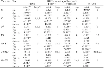
First, the order of integration of all relevant series was investigated, using a test of seasonal
integration (see Section 4.1.2) and the ADF test 4.1. Table 4 summarizes the seasonal
tests applied on the series collapsed into quarterly data. The non-rejection ofH01, together
with the rejection of bothH02and the joint hypothesisH03+04, suggests the presence of a
unit root at the zero frequency and no seasonal unit roots. Since there is a correspondence
between the quarterly and the monthly root at the zero frequency, not detecting seasonal
unit roots at the quarterly level is enough to consider that the series is affected only by
unit roots at the zero level and no testing at the monthly level is necessary. The table
shows that the null of seasonal unit roots can be rejected for all series,8 with the not very
surprising exception of T EM P.
After detecting with the seasonal approach the presence of only unit roots at the zero
frequency, the order of integration of the series was further tested using Dickey-Fuller-type
tests. Two auxiliaryDF regressions with and without a trend were used, and the optimal
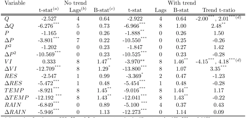
lag was chosen by an automatic sequential t-test. The results, shown in Table 5, reveal
that the trend component is not relevant in most cases. Table 5 shows that most variables
proved to beI(1). The hypothesis tests permit the rejection of the null of non-stationarity
of the differenced series at the 99% level of confidence. Once again, there are some doubts 8The test also permitted to reject the null hypothesis of seasonal unit roots in theIN F series, although
Table 4: Quarterly seasonal unit root test.
Variable Test HEGY model specification(a)
SEAS TREND STREND CONST t-stat(b)
Lags(c)
t-stat Lags t-stat Lags t-stat Lags
Q H01 -1.947 8 -2.379 0 -1.199 8 -2.929∗ 0
H02 -3.998∗∗ -3.684∗∗ -3.867∗∗ -3.848∗∗
H03+04 17.857∗∗ 6.176∗∗ 16.407∗∗ 6.485∗∗
P H01 -0.033 1,4,5 -1.136 0 -1.528 0 -1.108 0
H02 -4.116∗∗ -2.708∗∗ -2.795∗ -2.708∗∗
H03+04 12.143∗∗ 11.666 13.407∗∗ 11.701∗∗
P2 H
01 0.044 1,4,5 -1.237 0 -4.016∗∗ 4 -1.124 0
H02 -4.455∗∗ -2.750∗∗ -3.475∗∗ -2.743∗∗
H03+04 14.219∗∗ 12.233∗∗ 20.187∗∗ 12.194∗∗
V I H01 1.181 0 -0.787 1 0.311 0 -0.791 1,5
H02 -3.172∗∗ -0.418 -3.051 -0.829
H03+04 6.711∗∗ 0.332 6.604 0.744
RES H01 -2.970∗ 6 -2.643 3,5,7 -3.549∗ 0 -2.732∗ 5,6
H02 -3.177∗∗ -4.419∗∗ -4.299∗∗ -3.291∗∗
H03+04 15.982∗∗ 2.785∗ 7.027∗∗ 13.050∗∗
T EM P H01 -2.419 0 -3.401∗ 2,3,8 -2.399 0 -3.800∗∗ 2,3,6,7,8
H02 -2.133 -1.281 -2.111 -1.057
H03+04 8.117∗∗ 0.040 7.850∗∗ 0.280
RAIN H01 -2.062 4 -1.888 0 -2.775 2,4,8 -1.779 0
H02 -1.674∗ -1.674∗ -3.193∗∗ -1.677∗
H03+04 2.437∗ 2.437∗ 7.753∗∗ 2.400∗
(a) Test specifications: SEAS (Seasonal dummies + constant) TREND (Constant + trend) STREND
(Seasonal dummies + constant + trend) CONST (constant only)
(b) HEGY estimates,∗∗ and∗denote a t-ratio significant at the 5% and 10%
Table 5: Augmented Dickey-Fuller unit root tests.
Variable No trend With trend
t-stat(a) Lags(b) B-stat(c) t-stat Lags B-stat Trend t-ratio
Q -2.527 4 0.64 -2.922 4 0.64 -2.00∗∗∗, 2.01∗∗∗(d)
∆Q -6.276∗∗∗
5 0.73 -6.966∗∗∗
8 1.00 2.48∗∗ P -1.165 0 0.26 -1.888∗∗ 0 0.26 1.50
∆P -3.801∗∗∗ 7 0.22 -10.550∗∗∗ 0 0.25 -0.26
P2 -1.202 0 0.23 -1.847 0 0.27 1.42 ∆P2 -10.569∗∗∗ 0 0.23 -10.525∗∗∗ 0 0.23 -0.28
V I 0.333 8 1.47∗∗
-3.970∗∗ 8 1.46∗∗
-4.15∗∗∗
, 4.18∗∗∗(d)
∆V I -12.709∗∗∗
8 1.29∗
-13.800∗∗∗
8 1.07 3.35∗∗∗ RES -2.547 1 0.99 -3.369∗ 2 0.47 -1.23
∆RES -5.472∗∗∗ 1 0.48 -5.454∗∗∗ 1 0.48 -0.28
T EM P -8.921∗∗∗ 8 1.45∗∗ -9.016∗∗∗ 8 1.44∗∗ 1.17
∆T EM P -12.192∗∗∗
8 1.43∗∗
-12.041∗∗∗
8 1.43∗∗
-0.22
RAIN -6.849∗∗∗
0 0.89 -5.100∗∗∗
4 0.37 0.43
∆RAIN -5.946∗∗∗ 0 1.13 -12.273∗∗∗ 0 1.14 0.09
(a) t-ratio of estimates ***,∗∗ and∗denote a t-ratio significant at the 1%, 5% and 10%
(b) The number of lags (with a maximum of 8) to be included was selected using the Ng-Perron sequential-t test
(c) Bartlett’s (B) statistic of a cumulative periodogram white-noise test (H0: error is white noise) (d) This series exhibited a quadratic trend rather than a linear trend.
about the climate variables. T EM P appears to be stationary, but the seasonal unit root
tests did not reject the hypothesis of seasonal roots, so this variable should be considered
with caution, since it might be I(0,1). In the case of RAIN, we also see that the series
might actually be stationary in levels also at all frequencies, I(0). Since a definite claim
cannot be made that the climatic variables are nonstationary, their introduction in the
co-integration relationship and error-correction model cannot be understood in the same
way as the remaining variables. For this reason, an alternative model that accounts for
seasonality using only the binary variable SU M is also reported.9
The augmentation of the basic DF regression with extra lags (in Section 4.1) was
9A model (not reported but available upon request) based on a co-integration equation that did not
include neitherSU M nor the climatic variables (T EM P andRAIN) resulted in very similar price elast-icities (see Section 5.5) but slightly worse fit than the models that include seasonal variables. This, of course, confirms the intuition that the seasonal variables do not substantially affect the long-run dynamics
motivated by the need to generate iid errors. The number of lags was selected using
an Ng-Perron (1995) sequential-t test. A maximum of 8 lags was considered, given the
small sample size. A cumulative periodogram white-noise test was used to check that the
error was white noise in the unit root test regressions.10 An alternative solution is the
Phillips and Perron (1988) test (P P), which uses the same models asDF but, instead of
lagged variables, employs a non-parametric correction (Newey and West, 1987) for serial
correlation. The critical values for both the Dickey Fuller and Phillips Perron tests have
the same distributions (critical levels are reproduced in Hamilton, 1994). In principle,
the P P tests should be more powerful than the ADF ones, so the unit root tests were
conducted using both. The results of the P P test are not reported, but available upon
request.
5.2
Further unit root tests
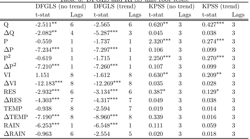
As described in Section 4.1.1, the conclusions of the Dickey-Fuller type tests can be suspect
in small samples and when the possibility of structural breaks has to be considered. A
DF GLS (ERS) test was used to confirm the nonstationarity of the main series in the
model. Since it is more powerful than the basic Dickey Fuller tests, this test will more
easily reject the null of nonstationarity. A KP SS test was also conducted to test the
alternative hypothesis of stationarity of the series. The results of both types of tests, in
Table 6, show no relevant differences with respect to those described in Section 5.1.
Similarly, structural breaks in the model’s series could affect the conclusions of the unit
root tests, above all because of the effects of the drought and the conservation measures
adopted by the water utility. For this reason the Clemente et al. (1998)’s tests, which
10In the case of T EM P and V I there were some doubts about whether the error had been whitened.
Table 6: DFGLS and KPSS unit root tests.
DFGLS (no trend) DFGLS (trend) KPSS (no trend) KPSS (trend) t-stat Lags t-stat Lags t-stat Lags t-stat Lags Q -2.511∗∗ 6 -2.565 6 0.620∗∗ 3 0.427∗∗∗ 3
∆Q -2.082∗∗ 4 -5.287∗∗∗ 3 0.045 3 0.038 3
P -0.559 1 -1.737 1 2.320∗∗∗ 3 0.274∗∗∗ 3
∆P -7.234∗∗∗ 1 -7.297∗∗∗ 1 0.106 3 0.099 3
P2 -0.619 1 -1.715 1 2.250∗∗∗ 3 0.270∗∗∗ 3
∆P2 -7.210∗∗∗ 1 -7.260∗∗∗ 1 0.107 3 0.099 3
VI 1.151 8 -1.612 8 0.630∗∗ 3 0.209∗∗ 3
∆VI -12.183∗∗∗ 8 -12.269∗∗∗ 8 0.035 3 0.028 3
RES -2.932∗∗∗ 6 -3.134∗∗∗ 6 0.387∗ 3 0.129∗ 3
∆RES -4.303∗∗∗ 7 -4.317∗∗∗ 7 0.049 3 0.038 3
TEMP -0.938 8 -2.594 7 0.019 3 0.014 3
∆TEMP -7.190∗∗∗ 8 -8.960∗∗∗ 8 0.339 3 0.016 3
RAIN -6.253∗∗∗ 1 -6.548∗∗∗ 1 0.111 3 0.059 3
∆RAIN -0.963 6 -2.554 5 0.020 3 0.018 3
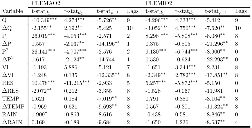
allow for either one (CLEM AO1andCLEM IO1) or two (CLEM AO2andCLEM IO2)
structural breaks in the time series,11 were used to obtain further confirmation of the
nonstationarity of the main series considered. The results (Tables 7 and 8) confirm that
most series exhibit evidence of structural breaks. However, even when these are considered,
there is not enough evidence to reject the null of nonstationarity.12
Since the additional unit root testing supports the notion that, with the exception of
the climatic variables, the series used in the demand model are nonstationary, the next
step is to analyze the co-integrating relationships among those variables.
5.3
Co-integration regression analysis
All the series infirst-differences are stationary, so the next step is to check that there is a
long-run equilibrium relationship between the variables. This requires an extension of the
11These were implemented in Stata usingclemao2andclemio2, respectively (Baum, 2005).
12Although the case of nonstationarity for theQseries is less clear now that what the tests in Section
Table 7: CLEMAO1 and CLEMIO1 unit root tests.
CLEMAO1 CLEMIO1
Variable t-statd1 t-statρ−1 Lags t-statd1 t-statρ−1 Lags
Q -8.345∗∗∗ -1.407 8 -4.274 -5.579∗∗ 3
∆Q -1.008 -6.447∗∗ 3 1.790∗ -6.767 8
P 26.786∗∗∗ -2.121 2 5.236∗∗∗ -5.376∗∗ 0
∆P 0.411 -12.216∗∗ 1 -0.763 -17.668∗∗ 0
P2 25.907∗∗∗ -1.993 2 5.215∗∗∗ -5.364∗∗ 0
∆P2 0.420 -12.094∗∗ 1 -0.738 -17.508∗∗ 0
VI 5.789∗∗∗ -3.499 6 2.567∗∗ -2.028 8
∆VI -0.839 -10.819∗∗ 8 -0.577 -12.731∗∗ 8
RES -2.979 -3.137 6 -2.074∗∗ -3.852 2
∆RES -0.970 -3.469 7 -0.326 -9.861∗∗ 0
TEMP 0.786 -7.373∗∗ 8 1.193 -7.874∗∗ 8
∆TEMP -0.838 -9.729∗∗ 8 0.628 -11.562∗∗ 8
RAIN 2.061∗∗ -7.822∗∗ 1 -0.006 -7.836∗∗ 0
∆RAIN 0.034 -9.308∗∗ 2 -0.421 -6.650∗∗ 8
Table 8: CLEMAO2 and CLEMIO2 unit root tests.
CLEMAO2 CLEMIO2
Variable t-statd1 t-statd2 t-statρ−1 Lags t-statd1 t-statd2 t-statρ−1 Lags
Q -10.349∗∗∗ 4.274∗∗∗ -5.726∗∗ 9 -4.296∗∗∗ 4.333∗∗∗ -5.412 9
∆Q -2.155∗∗ 2.192∗∗ -5.425 10 -3.052∗∗∗ 4.750∗∗∗ -7.620∗∗ 10
P 26.019∗∗∗ -4.053∗∗∗ -2.571 2 8.298∗∗∗ -5.808∗∗∗ -8.080∗∗ 8
∆P 1.557 -2.037∗∗ -14.196∗∗ 1 0.375 -0.805 -21.296∗∗ 8
P2 26.141∗∗∗ -4.707∗∗∗ -2.576 2 9.130∗∗∗ -6.744∗∗∗ -8.900∗∗ 0
∆P2 1.617 -2.124∗∗ -14.744 1 0.530 -0.924 -22.293∗∗ 0
VI -1.193 5.886 -5.121 7 -1.651 3.344∗∗∗ -2.231 8
∆VI -1.248 0.135 -12.335∗∗ 8 -2.349∗∗ 2.782∗∗∗ -13.851∗∗ 8
RES 10.478∗∗∗ -11.215∗∗∗ -2.933 5 5.257∗∗∗ -5.872∗∗∗ -5.150 0
∆RES -2.072∗∗ 0.212 -3.355 8 -1.528 -0.067 -11.981 0
TEMP 0.621 0.184 -7.019∗∗ 8 0.791 0.880 -8.104∗∗ 8
∆TEMP -0.969 0.621 -9.698∗∗ 8 0.567 -0.201 -11.324∗∗ 8
RAIN 1.909∗ -0.863 -8.616 8 -0.438 0.581 -8.846∗∗ 0
[image:26.612.100.534.456.677.2]linear relationship between water consumption and a series of variables that the economic
theory suggests appropriate. The model given by Equation (5) was extended into two
alternative models (time subscripts have been dropped to simplify the exposition):
Q=α+P +P2
+RES+V I+BAN+SU M+µ (7)
including the binary variable SU M instead of the climatic variables (see Section 3) and:
Q=α0+P +P2
+RES+V I+BAN+T EM P +RAIN+µ0 (8)
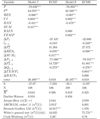
Table 9 shows the OLS estimated coefficients of each of the variables and their t
-statistics in these estimations. TheADF test shows that the hypothesis that the residuals
in Model 7 are non-stationary can be rejected. The relevant t-ratio is−5.62513 in the usual
test of a unit root and must be compared with the critical values provided by Engle and Yoo
(1987), which depend on the dimension of the time-series and on the number of variables
included in the model. The DW statistic is also higher than theR2, which suggests the
existence of the co-integration relationship.14 The long run price-elasticity calculated at
the means of price and quantity according to Model 7 is−0.491. All the variables present
the expected signs and are highly significant.
The ADF test shows that the hypothesis that the residuals in Model 8 are
non-stationary can be rejected too. The relevant t-ratio is−5.36415. TheDW statistic is again
13This value permits the rejection of the null of no co-integration at a 99% con
fidence level, but it is
achieved when the auxiliary regression includes no lags. Five lags are selected by Ng Perron’s sequential t-ratio and the Akaike Information Criterion test, yielding a t-statistic of -3.053 and one lag is selected by the Hannan-Quinn (1979) criterion, yielding a t-statistic of -3.804.
14An alternative co-integrating regression test (Sargan and Bhargava, 1983) uses the DW statistic from
the co-integrating regression. If the residuals are non-stationary, the DW statistic will approach zero as the sample size increases, so large values of the DW statistic suggest that a cointegrating relationship exists.
15This value permits the rejection of the null of no co-integration at a 99% con
fidence level, but it is
Table 9: Cointegration Models 7 and 8 and Error Correction equations ECM7 and ECM8.
Variable Model 7 ECM7 Model8 ECM8
P -78.629∗∗∗ -76.950∗∗∗
P2 64.070∗∗∗ 62.569∗∗∗ RES -0.066∗∗ -0.067∗∗
V I 0.003∗∗∗ 0.002∗∗∗
BAN -0.451∗∗ -0.473∗∗
SU M 0.317∗∗∗
RAIN 0.000
T EM P 0.002∗∗∗
∆Pt -37.437 -32.609
bεt−1 -0.218∗ -0.249∗∗
∆P2
t 31.264 27.572
∆RESt -0.076∗∗ -0.098∗∗∗
∆SU Mt 0.317∗∗∗
∆Pt−1 -71.006∗∗∗ -79.555∗∗∗
∆P2
t−1 54.729∗∗ 61.881∗∗∗
∆Qt−1 -0.273∗∗ -0.276∗∗
∆T EM Pt 0.004∗∗∗
∆RAINt 0.000
cons 26.489∗∗∗ 0.019 26.197∗∗∗ 0.019
ll -47.07 -7.233 -50.1 -3.197 N 108 106 108 106
R2 0.644 0.386 0.619 0.425 Durbin-Watson 0.919 0.856
Jarque-Bera (κ(2) =) 2.044 2.059 ARCH-LM, order( 1) (κ2(1)) 2.913∗ 0.001
Breusch-Godfrey LM (κ2
(1)) 16.917∗∗∗ 1.876
White’s general test (κ2
(1)(44)) 44.025 75.721∗∗
higher than the R2. The corresponding long run price-elasticity according to Model 8 is
−0.494, basically the same as the one obtained with Model 7. Once again, all variables
have the expected signs and are highly significant. The exception isRAIN, which presents
a positive sign, while we would normally expect more precipitation to reduce water use.
However, it cannot be rejected that its coefficient is null. According to theADF tests, the
null of no co-integration can only be rejected if the lag length of the auxiliary regression is
not optimally chosen. However, the value of theDW test and economic intuition suggest
that a long-run relationship would govern the variables concerned.
Since there are more than two nonstationary series involved in the model, there could
exist more than one co-integrating relationship. For this reason and in order to obtain
more definite evidence on the existence of a co-integrating regression, the Johansen and
Juselius maximum likelihood method for co-integration (see Johansen, 1988; Johansen and
Juselius, 1990; and Osterwald-Lenum, 1992, for details) was used to determine the number
of co-integrating relationships. The summarized results are shown in Tables 10 and 11.
The eigenvalues and the maximal eigenvalue and trace statistics for the VAR matrix are
shown as well as the relevant critical values. The null hypothesis of more than one
co-integrating relationship was rejected at the 1%level of significance in all cases, except in
the case of the trace test for Model 7, which rejects the null of no-cointegration only at
about the 15%. Likelihood-ratio and Wald test statistics for the exclusion of variables
from that co-integrating relationship were also conducted, and all variables included in
the co-integration tests were found relevant. Therefore, the Johansen tests support the
assumption of co-integration for both models.
Table 10: Model 7 Johansen-Juselius co-integration rank test.
H1:
H0: Max-lambda Trace Eigenvalues rank<=(r) statistics statistics (lambda) r (rank<=(r+1)) (rank<=(p=7)) .40067781 0 54.779285 115.46473 .2222569 1 26.895414 60.685446 .16540982 2 19.347149 33.790032 Osterwald-Lenum Critical values (99% interval):
Table/Case: 1∗ (assumption: intercept in co-integrating Equation)
H0: Max-lambda Trace 0 51.91 143.09 1 46.82 111.01 2 39.79 84.45 Table/Case: 1 (assumption: intercept in VAR)
H0: Max-lambda Trace 0 51.57 133.57 1 45.10 103.18 2 38.77 76.07 Sample: 1 to 108 N= 107
5.4
Error correction models
Since most of the evidence points towards the stationarity of the residuals of the
co-integrating regressions, their residuals can be introduced as error correction terms in two
error correction models. Thextvariables in Equation 6 are substituted byfirst differences
and lagged differences16 of the co-integrating variables. Thefirst error correction specifi
c-ation, ECM7 includes a summer variable, whereas the second model, ECM8 includes
T EM P and RAIN (although T EM P might suffer problems of seasonal unit roots and
it is dubious that T EM P and RAIN are nonstationary, so this second model should be
considered with caution). Table 9 reports the results of these OLS estimations. These
include lagged values of the differences of some variables. V I was left out of the ECM 16The signi
Table 11: Model 8 Johansen-Juselius co-integration rank test.
H1:
H0: Max-lambda Trace Eigenvalues rank<=(r) statistics statistics (lambda) r (rank<=(r+1)) (rank<=(p=8)) .58686628 0 94.586283 185.98108 .2725507 1 34.048574 91.394798 .23272295 2 28.345084 57.346224 Osterwald-Lenum Critical values (99% interval):
Table/Case: 1∗ (assumption: intercept in co-integrating Equation)
H0: Max-lambda Trace 0 57.95 177.20 1 51.91 143.09 2 46.82 111.01 Table/Case: 1 (assumption: intercept in VAR)
H0: Max-lambda Trace 0 57.69 168.36 1 51.57 133.57 2 45.10 103.18 Sample: 1 to 108 N= 107
models, since it showed problems of multicollinearity with the price variables and its
in-troduction made them non-significant. It is reasonable to assume that changes in income
tend to affect water use only in the long run, most likely through impacts on the
compos-ition of the capital stock. BAN was found non-significant too and it was removed from
the ECM regressions. The speed of adjustment towards equilibrium (bεt−1 in Table 9,
corresponding to (yt−1−θxt−1)in the notation used in Equation 2) is given by−0.218in
ECM7 and−0.249in ECM8. It can be seen that these error correction terms have the
expected negative sign and are both significant, which further supports the acceptance of
the co-integration hypothesis.
The Ramsey RESET-test (using powers of the fitted values of ∆Qt) shows that the
null hypothesis that Models ECM7 and ECM8 have no omitted variables cannot be
are normally distributed and are neither autocorrelated nor heteroskedastic in the error
correction equations. These include a Jarque-Bera (1980) test for normality of the
resid-uals; White’s (1980) general test statistic and Cook-Weisberg (1983) test,17 which uses
fitted values of ∆Qt, for heteroskedasticity; a Lagrange multiplier test for autoregressive
conditional heteroskedasticity (ARCH), based on Engle (1982); and a Breusch
(1978)-Godfrey (1978) LM test. They all present acceptable values, with the exception of the
Breusch-Godfrey LM test, which leads to the rejection of the null of non-autocorrelation
inECM7. An alternative model with extra lagged values of the price variables solves this
problem and yields a short-run elasticity of −0.073, as reported below. The results of this
additional augmented regression do not differ significantly from the ones reported and are
available upon request.
5.5
Price elasticities
The computation of short-run price elasticities (eSR) using the average price and water
consumption, yields the following results. Using ECM7 and the co-integration regression
in Model 7,eSR =−0.159(while the augmented model used to correct for autocorrelation
would yield eSR=−0.073) and the eLR =−0.494. Similarly, ECM7 and Model 7 yield
eSR=−0.101and eLR =−0.491.18
These estimates of price-elasticities confirm that residential water demand is inelastic
to its price, but not perfectly so. Almost all the papers published on residential water
demand agree on this result. Additionally these results confirm the intuition that
long-run elasticities are higher (in absolute values) than short-long-run ones (Dandy, et al., 1997;
Nauges and Thomas, 2003; Martínez-Espiñeira and Nauges, 2004) and also than most of
17Also known as Breusch-Pagan (1979) test for heteroskedasticity.
18A model based on a co-integration equation that did not include neitherSU Mnor the climatic variables
the measures that have been obtained in other European countries.19 The use of the
co-integration approach to model the demand for water yields rather sensible results and helps
to distinguish between the short-run effects and the long-run effects of pricing policies.
5.6
Wickens-Breusch one-step approach
The Engle-Granger procedure described above enjoys important attractive asymptotic
properties but it also suffers weaknesses. In finite samples, the parameter estimates are
biased. The extent of this bias can be severe, and will depend on omitted dynamics and
failure of the assumption of weak exogeneity among other things. The reasonable size
of the sample and the fact that the estimates agree with economic theory and previous
empirical research based on alternative econometric techniques suggest in principle that
this might be a minor problem in this case. Another problem, however, is that there is no
possibility to test the long run parameters.20 For these reasons, an additional regression
was run using the one-step Wickens-Breusch (1988) approach. The results are reported in
Table 12. The associated price-elasticities, calculated at the means of price and quantity
are eSR =−0.08 and eLR =−0.405in the model that uses SU M and eSR=−0.113 and
eLR =−0.514 in the model that uses T EM P and RAIN. The estimates are very close
to the ones calculated with the Engle-Granger approach, which suggests that they can be
accepted with more confidence. They also fall reasonably close to the values previously
obtained using alternative econometric techniques on data from the same city.
García-Valiñas (2002) estimated a price-elasticity of -0.25 for the first block of consumption and
-0.77 for the second block, while García-Valiñas (2005) estimated the price-elasticity as
19See Arbués et al. (2003) for a review of water demand studies with a special focus on European cases. 20The limiting distributions of theβparameters are non-normal and non-standard. Standard hypothesis
-0.49. Martínez-Espiñeira and Nauges (2004) found also that the short-run elasticity fell
around the value of -0.10, using a Stone-Geary demand specification.
Note that these values of price-elasticities compare well to those obtained in other
European areas, but are smaller than most values obtained in North America (see Arbués
et al., 2003 or Dalhuisen et al, 2003). In particular, studies based on discrete-continuous
choice models of water demand (Hewitt and Hanemann, 1995; Pint, 1999) obtain much
larger price elasticity estimates.21 This likely has to do with the fact that in Seville the
largest component of residential water use is associated with indoor water use, while,
contrary to many areas in the US, outdoor use is minimal. This confirms the notion that
price elasticities may be very different depending on the area of study, so policies should
be informed by studies based on at least similar areas.
6
Conclusions and suggestions for further research
This study is innovative in two aspects. This is the first time that co-integration and
error correction techniques are employed in the field of water consumption. Moreover,
the estimation of residential water demand using time-series monthly data is still rather
uncommon in Europe. The application of these techniques to monthly data to the case
of Seville leads to satisfactory results. The fit of the Granger co-integration relationship
between water use and the variables that should be expected to influence it in the long
run and of the error correction models is quite good. The dynamic properties of the series
were analyzed using different approaches and two alternative specifications for the water
demand functions were used. However, the results in terms of price elasticities, most of
all in the short run, are remarkably close. This robustness to specification and testing 21However, note that Cavanagh et al. (2002) found smaller elasticities using a similar methodology for
Table 12: Wickens-Breusch one-step cointegration regressions, Models 7 and 8 (dependent variable: ∆Qt−1).
Model 7 Model 8
Pt−1 -14.826 -12.811 Qt−1 -0.197∗∗ -0.219∗∗∗ P2
t−1 12.205 10.122
∆Qt−2 0.226∗∗
BANt−1 -0.186∗ -0.286∗∗∗
∆Pt−1 -4.904∗∗ -6.274∗∗
∆SU Mt 0.236∗∗
∆SU Mt−1 -0.228∗∗
∆RESt -0.054∗ -0.071∗∗
∆Pt−2 68.637∗∗∗
∆P2
t−2 -53.915∗∗ SU Mt−1 0.121
∆Qt−2 -0.417∗∗∗
∆T EM Pt−2 0.004∗∗∗
RAINt−1 0.000∗∗
∆IN Ft−1 -0.558∗
∆RAINt 0
∆BANt 0.363
CON S 5.664∗ 5.354
R2 0.4553 0.4207
N 105 106
F 8.25∗∗∗ 7.35∗∗∗
RESET 0.55 1.75 Jarque-Bera normality test (κ(2)) 21.49∗∗∗ 5.669∗
ARCH-LM test statistic (κ2
(1)) 3.154 0.0265371 Breusch-Godfrey LM-statistic (κ2(1)) 8856157 1.717
White’s general test statistic (κ2(1)(44)) 101.277∗ 89.592∗
procedures leads to confidently accept the main results.
The estimates of the price effects obtained are less than one in absolute value, which
confirms the inelasticity of household demand with respect to the price of water. As
predicted by the theory, the long-run price elasticities are greater, in absolute value, than
their short-run counterparts.
The measure of the impact of pricing policies on the behavior of households depending
on the changes that these policies introduce in the tariffstructure is still an open research
area. The long-run effects of water pricing on water use should be investigated using other
datasets, involving different regions, and, if possible, longer time-series or panel data.
Ideally, studies should be conducted at the individual level, with observations linked to
the ownership and frequency of renewal of capital stock.
References
Agthe, D. E. and R. B. Billings (1980). Dynamic models of residential water demand.
Water Resources Research 16(3), 476—480.
Agthe, D. E., R. B. Billings, J. L. Dobra, and K. Rafiee (1986). A simultaneous equation
demand model for block rates.Water Resources Research 22(1), 1—4.
Andrews, D. and E. Zivot (1992). Further evidence on the Great Crash, the Oil Price
shock, and the unit-root hypothesis.Journal of Business and Economic Statistics 10,
251—270.
Arbués, F., M. A. García-Valiñas, and R. Martínez-Espiñeira (2003). Estimation of
res-idential water demand: A state of the art review.Journal of Socio-Economics 32(1),
Banerjee, A., R. Lumsdaine, and J. H. Stock (1992). Recursive and sequential tests
of the unit-root and trend-break hypotheses: Theory and international evidence.
Journal of Business and Economic Statistics 10(3), 271—287.
Baum, C. (2000). Tests for stationarity of a time series. Stata Technical Bulletin 57,
sts15.
Baum, C. F. (2001). The language of choice for time series analysis? The Stata
Journal 1(1), 1—16.
Baum, C. F. (2005). CLEMAO_IO: Stata module to perform unit root tests with one
or two structural breaks. Statistical Software Components S444302, Boston College
Department of Economics, revised 17 Jun 2005.
Beaulieu, J. J. and J. A. Miron (1993). Seasonal unit roots in aggregate U.S. data.
Journal of Econometrics 55(1), 305—328.
Beenstock, M., E. Goldin, and D. Nabot (1999). The demand for electricity in Israel.
Energy Economics 21(2), 168—183.
Bentzen, J. (1994). Empirical analysis of gasoline demand in Denmark using
cointegra-tion techniques.Journal of Energy Economics 16(2), 139—143.
Billings, R. B. (1982). Specification of block rate price variables in demand models.
Land Economics 58(3), 386—393.
Breusch, T. S. (1978). Testing for autocorrelation in dynamic linear models.Australian
Economic Papers 17, 334—355.
Breusch, T. V. and A. R. Pagan (1979). A simple test for heteroskedasticity and random
coefficient variation.Econometrica 47(5), 1287—1294.
Household water demand under increasing-block prices. FEEM Working Paper No.
40.2002.
Chicoine, D. L. and G. Ramamurthy (1986). Evidence on the specification of price in
the study of domestic water demand. Land Economics 62(1), 26—32.
Clemente, J., A. Montañés, and M. Reyes (1998). Testing for a unit root in variables
with a double change in the mean.Economics Letters 59, 175—182.
Cook, R. D. and S. Weisberg (1983). Diagnostics for heteroscedasticity in regression.
Biometrika 70(1), 1—10.
Dalhuisen, J. M., R. Florax, H. L. F. de Groot, and P. Nijkamp (2003). Price and
income elasticities of residential water demand: Why empirical estimates differ.
Land Economics 79(2), 292—308.
Dandy, G., T. Nguyen, and C. Davies (1997). Estimating residential water demand in
the presence of free allowances.Land Economics 73(1), 125—139.
Dickey, D. A. and W. A. Fuller (1979). Distribution of the estimators for autoregressive
time series with a unit root.Journal of the American Statistical Association 74(366),
427—431.
Dickey, D. A. and W. A. Fuller (1981). Likelihood ratio statistics for autoregressive
processes.Econometrica 49(4), 1057—1072.
Eguía, B. and C. Echevarría (2004). Unemployment rates and population changes in
Spain.Journal of Applied Economics VII(1), 47—76.
Elliott, G., T. J. Rothenberg, and J. H. Stock (1996). Efficient tests for an autoregressive
unit root.Econometrica 64, 813—836.
analysis using cointegration techniques. Energy Economics 17(3), 249—253.
EMASESA (1997). Crónica de una Sequía. Sevilla: EMASESA.
EMASESA (2000). Water demand management: The perspective of EMASESA.
Tech-nical report, EMASESA.
Engle, R. (1982). Autoregressive conditional heteroskedasticity with estimates of the
variance of United Kingdom inflation. Econometrica 50(4), 987—1007.
Engle, R. and C. W. J. Granger (1987). Cointegration and error correction:
Represent-ation, estimation and testing.Econometrica 55(2), 251—76.
Engle, R. F., C. W. J. Granger, and J. S. Hallman (1989). Merging short and long
run forecasts: An application of seasonal cointegration to monthly electricity sales
forecasting.Journal of Econometrics 40(1), 45—62.
Engle, R. F. and B. S. Yoo (1987). Forecasting and testing in co-integrated systems.
Journal of Econometrics 35(1), 143—159.
Fouquet, R. (1995). The impact of VAT introduction on UK residential energy demand.
An investigation using the cointegration approach. Energy Economics 17(3), 237—
247.
Franses, P. (1991). Seasonality, nonstationarity and forecasting of monthly time series.
International Journal of Forecasting 7, 199—208.
García-Valiñas, M. Á. (2002). Residential water demand: The impact of management
procedures during shortage periods. Water Intelligence Online 1(May).
García-Valiñas, M. A. (2005). Efficiency and equity in natural resources pricing: A
proposal for urban water distribution services. Environmental and Resource