Munich Personal RePEc Archive
Asymmetries in information processing
in a decision theory framework
Santos-Pinto, Luís
Universidade Nova de Lisboa
8 January 2003
Online at
https://mpra.ub.uni-muenchen.de/3146/
Asymmetries in Information Processing
in a Decision Theory Framework
†Luís Santos-Pinto
Universidade Nova de Lisboa, Departamento de Economia Campus de Campolide, PT-1099-032, Lisboa, Portugal
Email address: [email protected]
This version: April 27, 2007
Abstract
Research in psychology suggests that some individuals are more sensitive to positive than to negative information while others are more sensitive to nega-tive rather than posinega-tive information. I take these cogninega-tive posinega-tive-neganega-tive asymmetries in information processing to a Bayesian decision-theory model and explore its consequences in terms of decisions and payoffs. I show that in mono-tone decision problems economic agents with more positive-responsive informa-tion structures are always better off, ex-ante, when they face problems where payoffs are relatively more sensitive to the action chosen when the state of nature is favorable.
JEL Classification Numbers: A12, D81. Keywords: Information Processing; Decision Theory.
†This paper is part of my Ph.D. dissertation in University of California, San Diego.
1
Introduction
Information is a key component of most types of economic behavior. When we make our investment decisions, choose what career to follow, decide what type of health insurance coverage we want to have, when to retire, or what is the best schooling district for our kids, we are faced and have to process a wide variety of information and data that may come from published sources, past personal experience, or advice from relatives, friends and experts.
Research in psychology suggests that many individuals are more sensitive to positive than to negative information. According to Matlin and Gawron:
Many individuals (...) recognize pleasant stimuli faster; they judge pleasant stimuli to be more frequent; they use pleasant words more often; they supply a greater number of free associates to pleas-ant stimuli; they recall pleaspleas-ant items more accurately, they recall pleasant items earlier in a list; and they process pleasant information more rapidly. (Matlin and Gawron, 1979, pp. 41)
There is also evidence that other individuals are more sensitive to negative than to positive information. According to Lewicka, Czapinski, and Peeters, these individuals have:
(...) stronger cognitive curiosity manifested for negative than for positive stimuli (Fiske, 1980), higher linguistic sophistication for negative than for positive category labels (Clark and Clark, 1977), higher informativeness of negative than of positive personality trait labels (Czapinski, 1986), more rational and normatively appropriate character of inferences applied to negative than to positive targets (Lewicka, 1989). (Lewicka, Czapinski, and Peeters, 1992, pp. 426)
This papers incorporates asymmetries in information processing in a Bayesian decision-theory model and explore its consequences in terms of decisions and payoffs. I assume that while some people areendowed with positive-responsive information processing technologies (from now abbreviated to IPTs) others are endowed with negative-responsive IPTs. This assumption is my main departure from standard decision-theory. Individuals endowed with positive-responsive IPTs have an advantage in processing favorable information while those en-dowed with negative-responsive IPTs have an advantage in processing unfavor-able information.
with more positive-responsive IPTs. Thus, individuals endowed with these types of IPTs are not systematically mistaken, they just happen to have different characteristics that determine the way they view the world.
I propose precise definitions of more positive-responsive distribution of be-liefs and more positive-responsive information structures. I show that in mono-tone decision problems decision-makers with more positive-responsive (negative-responsive) information structures are always better off, ex-ante, when they face problems where payoffs are relatively more sensitive to the action chosen when the state of nature is favorable (unfavorable).
Just as a person with a highly sensitive sense of sound has an advantage in music (and may turn out to be a music performer or a composer) or a person with a highly sensitive sense of taste has an advantage in cooking (and may turn out to be a chef), an individual with a positive-responsive (negative-responsive) information structure has an advantage in decision problems where payoffs are relatively more sensitive to the action chosen when the information about the state of nature is favorable (unfavorable).
The paper proceeds as follows. Section 2 sets-up of the decision problem. Section 3 explains how information structures can be compared. Section 4 in-troduces the positive-responsive order for posterior beliefs. Section 5 inin-troduces the set of incremental return functions associated with the positive-responsive order for posterior beliefs. Section 6 describes the main result and an economic application. Section 7 concludes the paper. Proofs of propositions are in the Appendix.
2
Set-up
Consider a Bayesian decision-theory framework where a decision-maker must choose an action or control variable (effort, output, prices) in order to maximize expected utility, which depends of both the control variable and of a random variable, or state of nature, that is not controlled by the decision-maker. Before choosing the control variable the decision-maker obtains information concerning the random variable. This information leads the decision-maker to update her beliefs about the state of nature and therefore make better decisions by com-parison with a situation where the decision maker is only in possession of his prior probability assessment of the realization of each state of nature.
The timing of the model is as follows:
1. Nature draws a state realization unobservable by the decision-maker;
2. Nature draws an imperfect signal about the true state realization;
3. The decision-maker processes the signal according to her information pro-cessing technology;
5. The payoffto the decision-maker is determined jointly by the action chosen and the state of nature realization.
Thus, for any two decision-makers endowed with different information pro-cessing technologies that face the same signaling technology, the one endowed with a “more positive-responsive” information processing technology processes signals in such a way that she ends up with a “more positive-responsive” in-formation structure than the decision-maker endowed with the “less positive-responsive” information processing technology. That is, decision-makers en-dowed with positive-responsive IPTs have positive-responsive information struc-tures and decision-makers endowed with responsive IPTs have negative-responsive information structures. Since, for all purposes, all that matters for individuals to make decisions is their information structures I do not need to model information processing technologies.1
The decision problem is composed of the followingfive elements.
1. A probability space(Ω,B, µ), whereΩis the set of possible realizations of the state of nature, withΩ= [a, b]⊂<,Bis the Borelσ-field ofΩandµ is a probability measure on(Ω,B), withµ(Ω) = 1.
2. Two real-valued random variablesXandW,whereXis the signal function with typical realizationx⊂X,withX = [c, d]⊂<,andW is the state of nature function with typical realizationω⊂Ω.
3. A joint probability distribution,F :Ω× X →[0,1],that will be called the decision-maker’s information structure and has generic element F(W = ω, X =x) or, in condensed notation,F(ω, x). Note that the two random variables,X andW, are fully characterized byF since fromF one can ob-tain (1) the marginal probability distribution of the signal,FX :X →[0,1],
with generic element FX(X =x) or, in condensed notation, FX(x), (2)
the decision maker’s prior beliefs or the marginal probability distribution of the state of nature,FW :Ω→[0,1],with generic elementFW(W =ω),
or, in condensed notationFW(ω), and (3) the decision maker’s posterior
beliefs after observing a signal realization X =xor the conditional dis-tribution of W given X =x, FW(·|x) : Ω→[0,1], with generic element
FW(W =ω|X =x)or, in condensed notation,FW(ω|x).
4. A set of actions,A,with typical element a∈A.
5. A payofffunction,w(ω, a), w:Ω× A→<.2
1Alternatively, I could have modelled an information system composed of three elements:
(1) a signaling technology (2) an information processing technology, and (3) an information structure. The information processing technology transforms signals into other signals, is unknown to and out of the control of the decision-maker. This approach is less parcimonious as the one I use here.
2To provide a better understanding of the payofffunction I compare it to the von
Neumann-Morgenstern utility function. LetXbe the set of consequences, outcomes or prizes, and let
Given thesefive elements I can define a the decision problem as the tuple D= (F, w, FW). I am now in a position where I can define the interim value of
the decision problemDgiven a signal realizationX =xand the ex ante value of a decision problemD. The interim value of the decision problemD given a signal realizationX =xis given by the expression
max a∈A
Z
Ω
w(ω, a)dFW(ω|x).
The ex ante value of the decision problemDis defined as
V (D) =
Z
X
⎡ ⎣max
a∈A
Z
Ω
w(ω, a)dFW(ω|x)
⎤
⎦dFX(x). (1)
LetW denote the set of all payoff functions and letFW denote the set of all prior probability distributions. A family of decision-makers will be defined by a pair(FW,WP)where FW ∈FW andWP stands for a set of payofffunctions
that have in common a certain propertyP. Furthermore, define the incremental return function as
r(ω) =w(ω, a0)−w(ω, a), ∀a0> a.
Most of the analysis that follows will focus on the incremental return function and not on the payofffunction directly. However, both functions are intimately related since the payoff of any action for any typical state of natureω can be written as a sum of incremental returns. Consider the case whereAis afinite set,A={a1, a2, . . . , an},then we have
w(ω, ak) = w(ω, a1) + [w(ω, a2)−w(ω, a1)] +. . .+ [w(ω, ak)−w(ω, ak−1)]
= w(ω, a1) +
k
X
i=2
ri(ω). (2)
Following Athey and Levin (1997) I let
R={g:Ω→<, gbounded and measurable},
and consider that a payofffunctionwhas anRQ incremental return function if
for anya0> awe haver(ω) =w(ω, a0)−w(ω, a)∈R
Q ⊂R.
The set of payoff functions with a RQ incremental return function will be
denoted by WRQ. For example, if the incremental return function is
nonde-creasing, then the set of payoff functions whose incremental return functions are nondecreasing will be denoted byWRN D.
toX.The outcome function specifies the consequence, outcome, or prize resulting from each state-action pair,x=ρ(ω, a).Letudenote the von Neumann-Morgenstern utility function, a mapping from Xto <.The payoff function is equivalent to the successive application of the outcome function and the von Neumann-Morgenstern utility function. That is,w(ω, a)≡
3
Comparison of Information Structures
Blackwell (1951,1953) has defined a partial order (we will denote it by%BL) on
the set of all information structures that says that an information structure,F0, is “more informative” than another, F, if and only if, for any payoff function and any prior distribution, the ex ante value of the decision problem when the decision-maker usesF0 is at least as large as the ex ante value of the decision problem when the decision-maker usesF,that is
F0%
BLF ⇔V(F0, w, FW)≥V(F, w, FW), ∀w∈W, ∀FW ∈FW.
This partial ordering of information structures says that more variable beliefs are desirable for any decision-maker, regardless of her attitude towards risk, since greater variability of beliefs means that signal realizations convey more information about the true state of nature.
The problem we face is of a different kind since we wish to find out in what types of economic environments does an individual with a more responsive information structure outperform an individual with a less positive-responsive information structure. To answer this question we need tofind the appropriate “more positive-responsive” order of information structures (we will denote it by %P R) and the right property of the incremental return function
(we will denote it byRP R),such that
F0%
P RF ⇔V(F0, w, FW)≥V(F, w, FW), ∀w∈WRP R, ∀FW ∈FW.
We need a notion of valuable information that is related to concrete economic environments and that necessarily does not hold across all economic environ-ments as Blackwell’s notion does. Thus, my “more positive-responsive” order will necessarily have to rank information structures that are not comparable using Blackwell’s “more informative” order.
4
PR Order for Posterior Beliefs
The PNA theory suggests that decision-makers endowed with negative-responsive IPTs are relatively more sensitive to perceiving unfavorable information than those endowed with positive-responsive IPTs. I need to turn this statement into an operational definition.
One possible interpretation is that a decision-maker endowed with a negative-responsive IPT is able to distinguish more accurately between different degrees of unfavorable information and is not able to distinguish as accurately between different degrees of favorable information when compared with a decision-maker endowed with a positive-responsive IPT. This interpretation has a direct transla-tion in terms of the dispersion of posterior beliefs: a “more positive-responsive” posterior distribution must have a greater dispersion of beliefs in favorable states of nature and a smaller dispersion of beliefs in unfavorable states than a “less positive-responsive” posterior distribution.
This suggests that an appropriate transfer of dispersion from the right to the left in a “more positive-responsive” posterior distribution will give us a “less positive-responsive” posterior distribution. However, this transfer of dispersion must be balanced. If we reduce the dispersion in the right side by a very small amount and increase the dispersion in the left side by a large amount it is most likely that the obtained (less positive-responsive) posterior distribution is overall more informative (in Blackwell’s sense) than the initial (more positive-responsive) posterior distribution. So, we wish that the transfer of dispersion in a distribution is done in such a way that it does not change its overall dispersion but simply changes the placement of dispersion.
One possible approach that obeys this criteria is to take as measure of over-all dispersion of a distribution its variance and restrict attention to comparing distributions that have the same mean and variance and differ only in terms of placement of dispersion. Basically, this approach says that a posterior distri-bution of beliefs is more positive-responsive than another if it has more upside dispersion of beliefs, or, a posterior distribution of beliefs is more negative-responsive than another if it has more downside dispersion of beliefs.
This approach parallels the one adopted by Menezes, Geiss, and Tressler (1980) for the characterization of increasing downside risk. Thus, my definition of a “more positive-responsive” distribution of posterior beliefs mirrors Menezes, Geiss, and Tressler’s concept of a “more upside risky” distribution of payoffs.3
Definition 1 The distribution of posterior beliefs FW(·|x0) is more
positive-responsive than FW(·|x) if FW(·|x) can be obtained from FW(·|x0) by a
se-quence of mean-variance-preserving transformations that shift dispersion of be-liefs from the right to the left.
Menezes, Geiss, and Tressler introduced to the economics literature the con-cept of a mean-variance-preserving transformation (MVPT): a combination of a
3A more negative-responsive (positive-responsive) distribution of posterior beliefs in my
mean-preserving spread (MPS) and a mean-preserving contraction (MPC) that, when applied to a distribution, preserves its variance. In a MVPT the MPS is applied everywhere before or after the MPC.4
Example: Table I illustrates a single MVPT that transforms fW (·|x0), the
more positive-responsive distribution, intofW(·|x),the less positive-responsive
distribution, by shifting dispersion of beliefs from the right to the left.
Table I
ω= 0 ω= 1 ω= 2 ω= 3 ω= 4
A 18/80 18/80 16/80 2/80 26/80
B 22/80 10/80 20/80 2/80 26/80
C 22/80 10/80 16/80 10/80 22/80
Line A shows the probability mass function fW(·|x0)Line B is obtained after
applying a 3-point MPS to the left offW(·|x0).5 Line C shows the probability
mass functionfW(·|x).Line C is obtained after applying a 3-point MPC to the
right of the probability mass function represented in line B. It is easy to check thatE[W|x0] =E[W|x] = 2andV[W|x0] =V[W|x] = 196/80.
Menezes, Geiss and Tressler’s Theorem 1 gives us an alternative way of characterizing the more positive-responsive order: one can say thatFW(·|x0)is
more positive-responsive thanFW(·|x)if and only if
E(W|x0) =E(W|x) (3) V (W|x0) =V (W|x) (4)
ω
Z
a t
Z
a
FW(z|x0)dzdt≥
ω
Z
a t
Z
a
FW(z|x)dzdt,∀ω ∈[a, b]. (5)
5
R
P RIncremental Return Functions
Having specified the more positive-responsive order on posterior beliefs we are now in a position were we can search for the appropriate property of the incre-mental return function that induces it. Thefirst thing to note is that inequality (5) is related to third-order stochastic dominance. To see this let us recall that the three stochastic dominance orders most commonly used in economics are
first, second and third-order stochastic dominance, FOSD, SOSD, and TOSD, respectively. These three orders, in our context, are defined as follows:
FOSD:FW(·|x0)%F OSDFW(·|x)ifFW(·|x0)6=FW(·|x)
andFW(·|x0)≤FW(·|x),∀ω∈[a, b]
4I will use the term MPS (and MPC) as defined by Landsberger and Meilijson’s (1990).
Their definition of a MPS avoids the drawbacks of Rothschild and Stiglitz’s (1970) definition.
5See Rasmusen and Petrakis (1992) for an illustration of the differences between a 4-point
SOSD:FW(·|x0)%SOSDFW(·|x)ifFW(ω|x0)6=FW(ω|x)
and
ω
R
a
FW(t|x0)dt≤
ω
R
a
FW(t|x)dt,∀ω∈[a, b]
TOSD:FW(·|x0)%T OSDFW(·|x)ifFW(ω|x0)6=FW(ω|x), E[W|x0]≥E[W|x]
and
ω
R
a t
R
a
FW(z|x0)dzdt≤
ω
R
a t
R
a
FW(z|x)dzdt,∀ω∈[a, b].
Thus, given conditions (3), (4), and (5) we see that if FW(·|x0).is more
positive-responsive thanFW(·|x),then FW(·|x0)is dominated by FW(·|x)by
TOSD, that is
FW(·|x0)%P RFW(·|x)⇒FW (·|x)%T OSDFW(·|x0). (6)
However, it is easy to see that the reverse is not true, that is,
FW(·|x)%T OSDFW(·|x0);FW(·|x0)%P RFW(·|x). (7)
Now, consider the following three classes of incremental return functions: R1={r(ω)∈R:rω(ω)>0}
R2={r(ω)∈R1:rωω(ω)≤0}
R3={r(ω)∈R2:rωωω(ω)≥0}.
The theorems that relate these three classes of incremental return functions withfirst, second, and third-order stochastic dominance can be stated as follows:
FW(·|x0)%F OSDFW(·|x)⇔E[r(W)|x0]≥E[r(W)|x],∀r(ω)∈R1
FW(·|x0)%SOSD FW(·|x)⇔E[r(W)|x0]≥E[r(W)|x],∀r(ω)∈R2
FW(·|x0)%T OSDFW (·|x)⇔E[r(W)|x0]≥E[r(W)|x],∀r(ω)∈R3
I am looking for a result that is similar to the third theorem.6 Defining
RP R={r(ω)∈R:rωωω(ω)≤0},
I can state the following result.
Proposition 1 The distribution of posterior beliefs FW(·|x0)is more
positive-responsive than FW (·|x) if and only if E[r(W)|x0] ≥E[r(W)|x] for all
in-cremental return functions in RP R, or
FW(·|x0)%P RFW (·|x)⇔E[r(W)|x0]≥E[r(W)|x],∀r(ω)∈RP R.
6See Hadar and Russel (1969) and Whitmore (1970). The third theorem says that if
FW(·|x0)dominatesFW(·|x)by TOSD then the expected incremental returns underFW(·|x0)
are weakly greater than the expected incremental returns underFW(·|x)for all incremental
The proof of this proposition is the proof of Theorem 2 in Menezes, Geiss and Tressler’s adapted to this context. To illustrate clearly the role that the imposition of equal means and equal variances plays I will show only how the if part is proved, that is how
FW(·|x0)%P RFW(·|x)⇒E[r(W)|x0]≥E[r(W)|x],∀r(ω)∈RP R.
By definition of expectation and using integration by parts one obtains7
E[r(W)|x0]
−E[r(W)|x] =−rω(b) [E(W|x)−E(W|x0)]
+1
2rωω(b){[V (W|x
0)
−V(W|x)] + [E(W|x)−E(W|x0)] [2b
−E(W|x0)
−E(W|x)]}
−
b
Z
a
rωωω(ω) ⎧ ⎨ ⎩ ω
Z
a t
Z
a
[FW(z|x0)−FW(z|x)]dzdt
⎫ ⎬ ⎭dω
(8)
Using the fact the more positive-responsive order imposes equal means,E(W|x0) = E(W|x), and equal variances,V(W|x0) =V(W|x), (8) simpli
fies to
E[r(W)|x0]−E[r(W)|x]
=− b
Z
a
rωωω(ω) ⎧ ⎨ ⎩ ω
Z
a t
Z
a
[FW(z|x0)−FW(z|x)]dzdt
⎫ ⎬
⎭dω. (9)
If the posterior distributionFW(·|x0)is more positive-responsive thanFW(·|x)
we know by (5) that the term in curly brackets in the right hand side of (9) is always nonnegative. So, for anyr(ω) ∈RP R we have that E[r(W)|x0] ≥
E[r(W)|x].
To give some intuition on the economic meaning of the sign of the third derivative of the incremental return function I introduce an example.
Example: Let the payofffunction be given by
w(ω, a) = 51.5
a−a
2
2 (5−ω)
1.5
, with ω≤5.
Its incremental return function is given byr(ω) =wa(ω, a) = 51.5−a(5−ω)
1.5
. We see that this incremental return function belongs to the set RP R since
rωωω(ω) =−38a(5−ω) −1.5
≤0.
LetΩ={0,1,2,3,4}andA=n1,(5/4)1.5,(5/3)1.5,(5/2)1.5,51.5o.In table II
I represent the payoffs associated with these actions and states
Table II
ω= 0 ω= 1 ω= 2 ω= 3 ω= 4
a= 1 5.6 7.1 8.6 9.8 10.7
a= (5/4)1.5 4.7 7.8 10.6 12.9 14.6
a= (5/3)1.5 −1.8 5.5 12.0 17.5 21.7
a= (5/2)1.5 −43.2 −18.3 3.6 22.1 36.4
a= 51.5
−573.8 −375.0 −119.8 −51.8 62.5
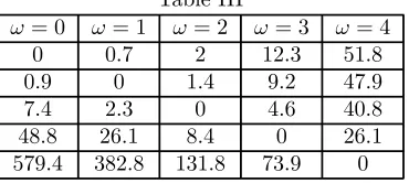
In table III I represent the incremental returns of the form
r(ω;a∗(ω), a) =w(ω, a∗(ω))−w(ω, a), wherea∗(ω) = max
a∈Aw(ω, a). Table III
ω= 0 ω= 1 ω= 2 ω= 3 ω= 4 0 0.7 2 12.3 51.8 0.9 0 1.4 9.2 47.9 7.4 2.3 0 4.6 40.8 48.8 26.1 8.4 0 26.1 579.4 382.8 131.8 73.9 0
By looking at the pattern of incremental returns in table III we see that if a decision-maker faces this problem and has noisy information about the state of nature it is worse not taking the no-noise optimal action when the state of nature is favorable (ω high) than when the state of nature is unfavorable (ω low). For example, whenω = 0the incremental return of taking action a= 1instead of taking actiona= (5/4)1.5is only 0.9 while whenω= 1 the incremental return of taking action a= (5/4)1.5 instead of taking action a= (5/3)1.5 is 2.3. As the state of nature becomes more favorable the incremental returns of taking the no-noise optimal actions increase. So, in this problem it is advantageous to have more accurate posteriors for high realizations ofω rather than for low realizations ofω,that is, a decision-maker faced with this problem will be better offwith a more positive-responsive information structure.
The previous example shows that the set of payofffunctions with incremental return functions with nonpositive third derivative can be interpreted as the set of payofffunctions whose payoffs are relatively more sensitive to the action chosen when the state of nature is favorable, in other words, payofffunctions where the cost of not taking the no-noise optimal actions is higher in favorable states than in unfavorable states.
6
PR Order for Information Structures
define a more positive-responsive order for information structures. For this purpose I introduce the following definition.
Definition 2 An information structureFis positive-responsive ordered if %P R
is a complete order on {FW(·|x)}x∈X, that is, for any x0 > x, FW(·|x0)%P R
FW(·|x).
Example: The posterior matrix shown in table IV induces a positive-responsive ordered information structure.
Table IV
x=.2 x=.4 x=.6 x=.8 x= 1 ω= 0 27/80 26/80 22/80 18/80 17/80 ω= 1 0/80 2/80 10/80 18/80 20/80 ω= 2 16/80 16/80 16/80 16/80 16/80 ω= 3 20/80 18/80 10/80 2/80 0/80 ω= 4 17/80 18/80 22/80 26/80 27/80
I restrict my attention to information structures that are positive-responsive ordered. By imposing this somewhat strong requirement the decision problem becomes monotone. This result is state formally in the next proposition.
Proposition 2 If w ⊂ WRP R and an information structure F is
positive-responsive ordered then there exists a decision rule α(x) that is nondecreasing in x.
This proposition tells us that if a decision-maker with a payoff function w⊂WRP R has a positive-responsive ordered information structure she has an
optimal decision rule that is monotone, that is, a decision rule where higher signals (more positive-responsive posteriors) lead to higher actions. The addi-tional structure of monotone decision problems enables us to derive necessary and sufficient conditions for decision-makers in certain economic environments to prefer more or less positive-responsive information structures.8
Before stating the main result of the paper I just have to define what a more positive-responsive information structure is.
Definition 3 Information structure F0 is more positive-responsive than infor-mation structure F, F0 %
P RF,if (i) F0 and F come from the same prior, (ii)
F0 and F are both positive-responsive ordered and (iii) for X0 and X being the two signals associated with information structures F0 and F, respectively, we have
F0
W (·|X0 ≥x)%P R FW(·|X ≥x), ∀x∈[0,1]. (10)
Condition (10), the monotone information order in Athey and Levin’s (1997), tells us that information structureF0 is more positive-responsive than informa-tion structure F if, on average, the more positive-responsive posterior beliefs
8Examples of monotone decision problems arise in many economic relevant contexts, such
(the ones induced by higher signal realizations) of information structureF0 are more dispersed than the more positive-responsive posterior beliefs of informa-tion structureF.I am now ready to state my mainfinding.
Proposition 3 Information structure F0 is more positive-responsive than in-formation structure F if and only if, for any payoff function inWRP R and any
prior distribution, the ex ante value of the decision problem when the decision-maker uses F0 is at least as large as the ex ante value of the decision problem when the decision-maker uses F,or
F0%
P RF ⇔V (F0, w, FW)≥V(F, w, FW), ∀w∈WRP R,∀FW ∈FW.
This proposition tells us that decision-makers with more positive-responsive information structures are always better off, ex-ante, when they face problems where payoffs are relatively more sensitive to the action chosen when the state of nature is favorable. Similarly, it tells us that decision-makers with more negative-responsive information structures are always better off, ex-ante, when they face problems where payoffs are relatively more sensitive to the action chosen when the state of nature is unfavorable.
To illustrate Proposition 3, consider a monopolist who faces cost uncertainty and that has a payoff function given byw(ω, q) = P(q)q−C(ω, q). The ex ante value of the monopolist’s decision problem is given by
V (D) =
Z
X
⎡ ⎣max
q≥0
Z
Ω
[P(q)q−C(ω, q)]dFW(ω|x)
⎤
⎦dFX(x).
Differentiating the payofffunction with respect to output we obtain the incre-mental return functionr(ω) =M R(q)−M C(ω, q). Differentiating the incre-mental return function with respect to the state of nature three times we get rωωω(ω) = −M Cωωω(ω, q). Proposition 3 tells us that if M Cωωω(ω, q) ≥ 0,
then a monopolist with a more positive-responsive information structure is al-ways better off ex ante than if he has a more negative-responsive information structure.
7
Conclusion
References
Athey, S. and Levin J. (2001). “The Value of Information in Monotone Decision Problems,” MIT Working Paper 98-24.
Blackwell, D. (1951). “Comparison of Experiments,”Proceedings of the Second Berkeley Symposium on Mathematical Statistics, 93-102.
Blackwell, D. (1953). “Equivalent Comparison of Experiments,” Annals of Mathematical Statistics, 24, 265-272.
Blackwell, D. and Girshick, M. (1954). Theory of Games and Statistical Deci-sions, Dover.
Borch, K. (1968). The Economics of Uncertainty, Princeton University Press. Fiedler, K., Fladung, U., and U. Hemmeter (1987). “A Positivity Bias in Person Memory,”European Journal of Social Psychology, Vol. 17, 243-246.
Hadar, J. and Russel W. (1969). “Rules for Ordering Uncertain Prospects,” American Economic Review, 59, 25-34.
Hirshleifer, J. and Riley, J. (1992). The Analytics of Uncertainty and Informa-tion, Cambridge University Press.
Laffont, J. (1989). The Economics of Uncertainty and Information, MIT Press. Landsberger, M. and Meilijson, I. (1990). “A Tale of Two Tails: An Alternative Characterization of Comparative Risk,” Journal of Risk and Uncertainty, 3, 65-82.
Lewicka, M., Czapinski, J., and G. Peeters (1992). “Positive-Negative Asym-metry or ‘When the Heart Needs a Reason,”’European Journal of Social Psy-chology, Vol. 22, 425-434.
Marschak, J. (1963). “The Payoff-Relevant Description of States and Acts,” Econometrica, Vol. 31, No. 4, 719-725.
Marschak, J. and Radner, R. (1972). Economic Theory of Teams, New Haven and London, Yale University Press.
Matlin, M. and Gawron, V. (1979). “Individual Differences in Pollyannaism,” Journal of Personality Assessment, 43, 411-412.
Menezes, C., Geiss, C., and Tressler (1980). “Increasing Downside Risk,” Amer-ican Economic Review, 70, No. 5, 921-932.
Milgrom, P. and C. Shannon (1994). “Monotone Comparative Statics,” Econo-metrica, Vol. 62, No. 1, 157-180.
Ormiston, M. (1992). “Deterministic Transformations: Some Comparative Statistics Results,” Decision Making under Risk and Uncertainty: New Mod-els and Empirical Findings, Geweke, J. Ed, 43-51.
Rasmusen, E. and Petrakis, E. (1992). “Defining The Mean-Preserving Spread: 3-PT Versus 4-PT,”Decision Making under Risk and Uncertainty: New Models and Empirical Findings, Geweke, J. Ed., 53-58.
Scholz, R. (1987). Cognitive Strategies in Stochastic Thinking, Theory and Decision Library, D. Reidel Publishing Company.
Shaked, M. and Shanthikumar, G. (1994). Stochastic Orders and their Applica-tions, Academic Press.
Shannon, C. (1995). “Weak and Strong Monotone Comparative Statics,” Eco-nomic Theory, 5(2), 209-227.
Whitmore, G. (1970). “Third Degree Stochastic Dominance,” American Eco-nomic Review, 60, 457-459.
8
Appendix
Proof of Equation (8): By definition of expectation we know that
E[r(W)|x0]−E[r(W)|x] = b
Z
a
r(ω) [dFW(ω|x0)−dFW (ω|x)]
= b
Z
a
r(ω) [fW(ω|x0)−fW(ω|x)]dω
Integrating by parts we obtain
E[r(W)|x0]
−E[r(W)|x] = |r(ω) [FW(ω|x0)−FW(ω|x)]|ba
−
b
Z
a
rω(ω) [FW(ω|x0)−FW(ω|x)]dω.
SinceFW(a|x0)−FW(a|x) = 0andFW(b|x0)−FW(b|x) = 0we have
E[r(W)|x0]−E[r(W)|x] =−
b
Z
a
rω(ω) [FW(ω|x0)−FW(ω|x)]dω.
Integrating by parts once again we have
E[r(W)|x0]
−E[r(W)|x] = −
¯ ¯ ¯ ¯ ¯ ¯
rω(ω) ω
Z
a
[FW (t|x0)−FW(t|x)]dt
¯ ¯ ¯ ¯ ¯ ¯ b a + b Z a
rωω(ω) ⎛ ⎝ ω
Z
a
[FW(t|x0)−FW(t|x)]dt
⎞ ⎠dω.
Integrating by parts the second term on the left hand side of the above equation we have
E[r(W)|x0]−E[r(W)|x] =−
¯ ¯ ¯ ¯ ¯ ¯
rω(ω) ω
Z
a
[FW(t|x0)−FW(t|x)]dt
¯ ¯ ¯ ¯ ¯ ¯ b a + ¯ ¯ ¯ ¯ ¯ ¯
rωω(ω) ω Z a ⎛ ⎝ t Z a
[FW(z|x0)−FW(z|x)]dz
⎞ ⎠dt ¯ ¯ ¯ ¯ ¯ ¯ b a − b Z a
rωωω(ω) ⎛ ⎝ ω Z a t Z a
[FW(z|x0)−FW(z|x)]dzdt
The above expression can be simplified to
E[r(W)|x0]
−E[r(W)|x] =−rω(b)
b
Z
a
[FW(ω|x0)−FW(ω|x)]dω
+rωω(b)
b Z a ⎛ ⎝ ω Z a
[FW(t|x0)−FW(t|x)]dt
⎞ ⎠dω
−
b
Z
a
rωωω(ω) ⎛ ⎝ ω Z a t Z a
[FW(z|x0)−FW(z|x)]dzdt
⎞ ⎠dω.
(11)
note that
b
Z
a
[1−FW(ω|x0)]dω=−a+E(W|x0)
and
b
Z
a
[1−FW(ω|x)]dω=−a+E(W|x),
imply that
b
Z
a
[FW(ω|x0)−FW(ω|x)]dω=E(W|x)−E(W|x0). (12)
Also, b Z a ⎛ ⎝ ω Z a
FW(t|x0)dt
⎞ ⎠dω= b
2
2 −bE(W|x
0) +1
2E
¡
W2
|x0¢,
and b Z a ⎛ ⎝ ω Z a
FW (t|x)dt
⎞ ⎠dω= b
2
2 −bE(W|x) + 1 2E
¡
W2
|x¢,
imply that b Z a ⎛ ⎝ ω Z a
[FW(t|x0)−FW(t|x)]dt
⎞ ⎠dω
=−b[E(W|x0)−E(W|x)] +1 2
£
E¡W2
|x0¢−E¡W2
Using the definition of variance we can write the above equation as
b
Z
a
⎛ ⎝ ω
Z
a
[FW(t|x0)−FW(t|x)]dt
⎞ ⎠dω
=1
2{[V(W|x
0)
−V (W|x)] + [E(W|x)−E(W|x0)] [2b
−E(W|x0)
−E(W|x)]}. (13)
Substituting (12) and (13) into (11) we obtain (8). Q.E.D. Proof of Proposition 2: This proof is a particular case of the proof of Lemma 1 in Athey and Levin’s (1997). DefineU(x, a) =RΩw(ω, a)dFW(ω|x)
and let the optimal action for signal realization X =x be defined as α(x) = arg maxa∈AU(x, a). We wish to show that if w ⊂WRP R and an information structureF is positive-responsive ordered then there exists an optimal decision rule,α(·), that is nondecreasing inx. We know from Shannon’s (1995) that if
X is a partially ordered set and U : X × A→<, where A⊂<, we have that
arg maxa∈AU(x, a) is nondecreasing in x if and only if U(x, a) satisfies the single crossing property ina. Thus, sinceX ⊂<,to prove this proposition we just need to show thatU(x, a)satisfies the single crossing property ina. Leta0 > a.We know that sincew
⊂WRP R thenr(ω) = w(ω, a0)−w(ω, a)∈
RP R. Given thatF is positive-responsive ordered we also have that ∀x0 > x,
FW(·|x0)%P RFW(·|x).By Proposition 1,FW(·|x0)%P RFW(·|x)implies
E[r(W)|x0] ≥ E[r(W)|x]
Z
Ω
r(ω)dFW(ω|x0)dω ≥
Z
Ω
r(ω)dFW(ω|x)dω
Z
Ω
[w(ω, a0)
−w(ω, a)]dFW(ω|x0) ≥
Z
Ω
[w(ω, a0)
−w(ω, a)]dFW(ω|x)
U(x0, a0)
−U(x0, a)
≥ U(x, a0)
−U(x, a)
The last inequality implies that∀a0 > a, U(x, a0)
−U(x, a)≥0⇒U(x0, a0) − U(x0, a)
≥0, ∀x0 > x, that is,U(x, a)satis
fies the single crossing property in
a. Q.E.D.
Proof of Proposition 3: This proof is a particular case of the proof of The-orem 3 in Athey and Levin’s (1997). Suppose A={a1, . . . , ai, . . . , an} and
Ω = {ω1, . . . ,ωj, . . . ,ωJ}, that is the action space and the space of state of
nature realizations isfinite.9 We need to show that for any optimal monotone
decision rule based on observing signal X, α(·), there is an alternative opti-mal monotone decision rule based on observing signalX0, α0(·), that makes a decision-maker ex-ante at least as well.
By Lemma 2 in Athey and Levin we know that (10) holds if and only if for all x∈[0,1]andr∈RP R
Z
Ω
r(ω)dFW0 (ω|X0≥x) Pr (X0≥x)≥
Z
Ω
r(ω)dFW(ω|X ≥x) Pr (X ≥x),
or
EW[r(ω)|X0 ≥x] Pr (X0≥x)≥EW[r(ω)|X ≥x] Pr (X ≥x). (14)
Let the optimal monotone decision rule associated with information structure F be defined by a set of cut points: x1 ≤ x2 ≤ . . .≤ xn+1, with α(x) =ai
whenxi< x < xi+1.The ex-ante expected payoffof usingα(·)with information
structureF is given by
V(F, w, FW,α) = m
X
j=1
n
X
i=1
w(ωj,α(xi))f(ωj, xi)
= m
X
j=1
n
X
i=1
w(ωj, ai)f(ωj, xi)
= m
X
j=1
[w(ωj, a1)f(ωj, x1) +. . .+w(ωj, an)f(ωj, xn)].
Making use of (2) we have that
V (F, w, FW,α) = m
X
j=1
{w(ωj, a1)f(ωj, x1) + [w(ωj, a1) +r2(ωj)]f(ωj, x2)
+ [w(ωj, a1) +r2(ωj) +r3(ωj)]f(ωj, x3) +. . .
+ [w(ωj, a1) +r2(ωj) +. . .+rn(ωj)]f(ωj, xn)} (15)
Collecting terms (15) becomes
V(F, w, FW,α) = m
X
j=1
{w(ωj, a1) [f(ωj, x1) +f(ωj, x2) +. . .+f(ωj, xn)]
+r2(ωj) [f(ωj, x2) +f(ωj, x3) +. . .+f(ωj, xn)]
+r3(ωj) [f(ωj, x3) +. . .+f(ωj, xn)] +. . .+rn(ωj)f(ωj, xn)
or
V(F, w, FW,α) = m
X
j=1
(
w(ωj, a1)
n
X
i=1
f(ωj, xi) +r2(ωj) n
X
i=2
f(ωj, xi)
+r3(ωj)
n
X
i=3
f(ωj, xi) +. . .+rn(ωj)f(ωj, xn)
or
V(F, w, FW,α) = m X j=1 ⎧ ⎪ ⎪ ⎨ ⎪ ⎪ ⎩
w(ωj, a1)f(ωj) +r2(ωj)
n
P
i=2
f(ωj, xi)
Pr (X≥x2)
Pr (X ≥x2)
+r3(ωj)
n
P
i=3
f(ωj, xi)
Pr (X ≥x3)
Pr (X ≥x3) +. . .+rn(ωj)
f(ωj, xn)
Pr (X ≥xn)Pr (X ≥xn)
⎫ ⎪ ⎪ ⎬ ⎪ ⎪ ⎭ or
V(F, u, FW,α) = m
X
j=1
u(ωj, a1)f(ωj) +
m
X
j=1
r2(ωj)
n
P
i=2
f(ωj, xi)
Pr (X ≥x2)
Pr (X≥x2)
+ m
X
j=1
r3(ωj)
n
P
i=3
f(ωj, xi)
Pr (X ≥x3)
Pr (X ≥x3)+. . .+
m
X
j=1
rn(ωj)
f(ωj, xn)
Pr (X ≥xn)Pr (X ≥xn)
or
V(F, w, FW,α) =E[w(W, a1)] +E[r2(W)|X≥x2] Pr (X ≥x2)
+E[r3(W)|X ≥x3] Pr (X ≥x3) +. . .+E[rn(W)|X≥xn] Pr (X ≥xn)
or,finally,
V (F, w, FW,α) =E[w(W, a1)] +
n
X
i=2
E[ri(W)|X ≥xi] Pr (X ≥xi). (16)
Let the optimal monotone decision rule associated with information structure F0 be defined by the set of cut points: x0
1 ≤x02 ≤. . .≤xn0+1, withα0(x) =ai
whenx0
i< x < x0i+1.The ex-ante expected payoffof usingα0(·)with information
structureF0 is given by
V (F0, w, F
W,α0) =E[w(W, a1)] +
n
X
i=2
E[ri(W)|X0≥xi] Pr (X0≥xi). (17)
Subtracting (16) from (17) we obtain
V(F0, w, FW,α0)−V(F, w, FW,α) = n
X
i=2
E[ri(W)|X0 ≥xi] Pr (X0 ≥xi)
−
n
X
i=2
E[ri(W)|X ≥xi] Pr (X ≥xi)
We see that (14) impliesV (F0, w, F