Real Time Dynamic State Estimation for
Power System
A. Thabet
Research Unit M.A.C.S University of Gabes, TUNISIAM. Boutayeb
Centre de Recherche CRANNancy University, FRANCE
M.N. Abdelkrim
Research Unit M.A.C.S University of Gabes, TUNISIAABSTRACT
This paper investigates a method for the state estimation of nonlinear systems described by a class of differential-algebraic equation (DAE) models using the extended Kalman filter. The method involves the use of a transformation from a DAE to ordinary differential equation (ODE). A relevant dynamic power systems model using decoupled techniques will be proposed. The estimation technique consists of a state estimator based on the EKF technique as well as local stability analysis. High performances are illustrated through a real time application on 5 buses test system with DSP device (Dspace DS1104).
Keywords
Power system dynamics, Extended Kalman Filter, convergence analysis, Time computing.
Nomenclature
M Inertia constant of the generator D Damping constant of the generator
δ mechanical rotor angle of the rotating machine ω mechanical angular velocity
ωs electrical angular velocity PM Mechanical power input Pj, Qj Nodal active and reactive power Pc,d Transit power
Ybus Nodal admittance matrix
, ij ij
G B real and imaginary terms of bus admittance matrix corresponding to ith row and jth column
N Total number of system buses ng Number of generator buses nl Number of load buses
PGi Electrical power supplied by the generator
,
i Vi
Phase and voltage at bus i1.
INTRODUCTION
As the power system becomes larger and more complex, real time monitoring and control become very significant in order to achieve a reliable operation of the power system. The Energy Management System (EMS) functions are responsible for this task of monitoring and control. Dynamic State estimation forms the backbone of the energy management system by providing a database of the real time state of the system for using in other EMS functions [1]. Hence, an efficient and accurate dynamic state estimation is a prerequisite for an efficient and reliable operation of power system.
State estimation in power system has mainly focused on Static State Estimation (SSE) from redundant measurement [2] [3]. However, to oversee an electrical power system in efficient, economic and secure manner, it is most important to be acquainted with the different dynamics states and then it’s Dynamic State Estimation (DSE) in electric power system, which apprises of the aforesaid information.
In designing a DSE, it is important to consider all algebraic and dynamic variables (bus voltages/phases and generators variables). The existing models are based on reducing the size of the model (linearized DAE) [4], linearization of the model [5]. To override the limitations of the existing models, a relevant and new model has been considered in this paper to model the dynamics of the power system based on the nonlinear DAE models proposed in [6]. We show that we can always rewrite the system with a nonlinear DAE form with explicit ODE to facilitate its implementation and operation. After validation of a robust dynamic model, it is extremely important to consider a robust estimator which reflects a reliable image in the terms of capacity as for estimation, robustness and stability. A large number of existing methods are based on:
The power system is considered as a quasi-static variables (voltages magnitudes and angles at network buses) and then applying a tracking estimator [7].
Definition of spaces of linear combinations and their algebraic complement for the calculation of the observer gains [8].
Most methods are based on the Kalman Filter for the reason of the complexity of the model [13] [14]. The advantages of the EKF are its simplicity, the fact that it is a recursive algorithm and so its computational load is modest [15] [16]. The EKF is suitable for real-time industrial-scale applications [17] with the development of the Digital Signal Processor devices.
The aim of this work is to show how a simple extended Kalman filter algorithm can solve the real time dynamic state estimation problem for power systems. Indeed, description of the network by a dynamic model leads us to have an idea about the transient behavior that plays a central role for monitoring and control design. We show that the dynamic model is always written as a nonlinear DAE. To develop useful and simple state estimator, we transform the obtained model to an augmented one written as a system of ordinary differential equations. Furthermore, to reduce the computational requirements and numerical instabilities, we show in the proposed decoupled dynamic model that the inverse of the Jacobian matrix can be approximated by the inverse of a block diagonal matrix using two sub-matrices of small dimensions. Thus, we propose a state estimator based on the Extended Kalman Filter with a study for stability analysis. In the last section, real time application on the 5 buses test system shows the relevance and efficiency of the proposed approaches.
2.
DYNAMIC POWER SYSTEM MODEL
The dynamics of a power system can be modeled with a combination of nonlinear differential equations and nonlinear algebraic equations. These sets of equations are often solved separately in different analysis techniques. The solution is accomplished in an iterative way, with the important feature that all the desired system characteristics are included. The general form of the DAE model is given as:( )
(
( ),
( ), ( ))
0
(
( ),
( ))
( )
(
( ),
( ))
d d d a
d a
d a
t
F
t
t
t
g
t
t
t
h
t
t
x
x
x
u
x
x
y
x
x
(1)
With: nd
d
x (t)
and( )
naa
x t
are respectively dynamic and algebraic states,( )
ndd
F t
a function representing the nonlinear differential equations,g
(.)
na represents the nonlinear algebraic constraints (equations),u t
( )
pthe control andy t
( )
m the output system. The problem with the system (1) is thatx t
a( )
does not appear explicitly.2.1
Problem Formulation
We consider these assumptions [6]:- The internal field currents are constant, providing the representation of the machine as a constant voltage behind the direct axis transient reactance. - The mechanical power provided by the prime mover
is constant and all dynamics of the prime mover are neglected.
- All generators are rotating at synchronous speed (steady state) and are round rotors.
- All generators in the system are identical, and therefore the inertia constant (Mi) along with the damping constant (Di) of each generator have the same value.
- The mechanical rotor angle is the same as the electrical phase angle of the voltage therefore δ now refers to the electrical angle. To further simplify the notation, the transient reactance is incorporated into the system Ybus, resulting in θi as generator terminal voltage phase and Vi as the terminal voltage magnitude.
If we take node 1 as reference, the set of equation of this network is given by [6]:
˙
, ,
: 0
: ( ( , , ) )
2
: ( , , ) 0
: ( , , ) 0
: ( , , )
i i
I
i i s
II s
i i M G i
I
i j j
II
i j j
q c d c d
f
f P P V D
M
g P P V
g Q Q V
y P P V
(2)
With:
1... g 1; ( g 1)...( g l); 1... ; , 1...
i n j n n n q m c d N,
the node 1 is taken as the reference and :
1
| || | [ cos( ) sin( )]
i
N
G i j ij i j ij i j
j
P V V G
B
Therefore the model (2) can be rewritten under this form:
( , , )
( , )
F x x
u
y
h x
with:
[ ,
, ,
] ,
T Mi,
{
}, (.)
[ ,
]
Ti i i i bus i j
P
x
V
u
Y
F
f g
M
and yPc d, where u and y will be respectively the control and the output of the system.
2.2
Semi-explicit DAE index 1
If at an equilibrium point, the system (1) is called semi-explicit [18], index-1 property requires that
g x
(
d,
x
a)
issolvable for
x
aanddet(
(
,
))
0
a
x d a
g
x
x
(tosimplifyx td( )xd,x ta( )xa):
0
(
,
)
(
,
)
0
(
,
)
F
d(
,
, )
(
,
)
d a
d a
x d a d x d a a
x d a d a x d a a
g
x
x
x
g
x
x
x
g
x
x
x
x u
g
x
x
x
(3)Where ( , ) ( , )
a
d a
x d a
a
g x x
g x x
x
and
( , ) ( , )
d
d a
x d a
d
g x x
g x x
x
In other words, the differentiation
index is 1, if, by differentiation of the algebraic equations with respect to time, an implicit ODE system results:
1
(
,
, )
(
,
)
(
,
)
(
,
,
)
d
d
F
F
a d
d d a
a x d a x d a d a
x
x
x u
x
g
x
x
g
x
x
x
x u
(4)Where 1( , ) a a
a
n n
x d a
g x x and
(
,
)
a dd
n n
x d a
g
x
x
.(
,
)
(
,
)
g
[ ]
a a
a
a a
x 1 x 2
d a
x d a
x 3 x 4
a
g
g
x
x
g
x
x
J
g
g
x
(5)With J is the Jacobian matrix used in the Load Flow calculation excepted for generators terms, which allows us to verify that this
det( (
g x
d,
x
a))
0
and g is solvable for anya
x
(the elements of this matrix are the components of the diagonal Jacobean matrix used in load flow).2.3
Proposed dynamic model
The basic idea is to extend the principle of decoupled algorithm used in Load Flow [3] and in SSE [2] to the dynamic model (and consequently to the DSE), but it apply only to the matrix
g
xa(
x
d,
x
a)
. In the dynamic model (4), matrix(
,
)
a
x d a
g
x
x
is formed by the differentiation of the algebraic constraints to the algebraic states and formed by the same elements of Jacobean matrix which are used for load flow calculation. In an equilibrium point (or around), we assume that the variation ofx
a is very small and can be approximated, with the same methodology used in Newton's algorithm to load flow calculation (same principle), by( 1) ( ) ( )
a a a
x n x n x n where:
1 ( )
[ ( )] ( , ) ( , )
( ) a d ( )
a x d a x d a
n
x n g x x g x x
V n P n
(6)
and
P n
( )
P
M( )
n
P n
G( )
and
s. Thesolution
x t
a( )
should always verify that calculated by loadflow (in permanent mode
x
a must be equal to 0 to verify the algebraic constraints). So we have the same formulation as that used for the load flow calculation and we can apply the principle of decoupled algorithms.With the same reasoning, we applied a change only to the matrix
(
,
)
a
x d a
g
x
x
in a similar way to that of the decoupled algorithm ((
,
) |
a
x d a Dec
g
x
x
):1 1
(
,
)
(
,
)
(
,
, )
(
,
) |
(
,
)
(
,
, )
a d
a d
a x d a x d a d d a
x d a Dec x d a d d a
x
g
x
x g
x
x F x
x u
g
x
x
g
x
x F x
x u
(7)
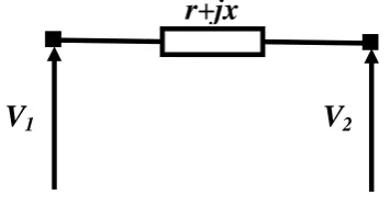
[image:3.595.87.265.617.716.2]We present in what follows the principle of decoupled algorithm used for load flow and SSE. Let us consider an electrical line model given at Fig. 1:
Fig 1. Schema of electrical line.
where the voltage
V
1 is supposed to be constant and the voltageV
2 is taken as the origin of phase with r and x arerespectively resistance and inductive reactance of line . We
have: 2 2
2
rQ
xP
V
and 2 22
rP
xQ
V
V
. In a highvoltage network, it is obvious that the phase
( )
depend primarily on the circulation of the active powers and that the modules of the nodal voltage (V) are mainly dependent on the circulation of the reactive powers becauser
x
. In theseconditions, we can approximate
and
V
by 2 2xP
V
and2 2
xQ
V
respectively. These approximations allow us to cancelsub matrix
[
2]
a
x
g
and[
3]
a
x
g
, therefore obtaining a reduced dimensions system [20]. We can thus write this matrix in the following simplified form:1
4
1 4
0 ( , ) |
( , ) |
0
0 [ ]
0
a a
a
x
d a Dec
x d a Dec
x a
Dec
g
g x x
g x x
g x
j J
j
(8)
To validate the proposed dynamic decoupled model, we tested the OM and proposed DM for 100 simulations while varying the initial values in a random way (variation of
20%
with respect to the actual initial values) in IEEE 3 buses test system. We put on Table 1 the relative error given by (9) wherex
realis generated by using the Toolbox SimPowerSystems of MATLAB®.
/
real OM DM
real
x x
x
‖ ‖
‖ ‖ (9)
Table 1. Relative error (%) and computing time with random initial
OM DM
Relative error 4.133 % 2.679%
Computing Time 1.72 s 1.24s
As we can see (line 2 of Table 1), the proposed decoupled model (DM) converge with an accurate precision than ordinary model (OM). Moreover, the results show that the computing time is better using DM which permits to implement more effectively this model for real time application.
For the calculation of
x
a, the mathematical expression are given in (10.a) for DM and in (10.b) for OM.1 1
0
( , , )
0
j i
j i
V
a d d a
P P
x F x x u
V Q Q
(10.a)
where i
j
i P P
and i
j
i Q Q
.
r+jx
1 1 1
2 3
( ) 0
( , , )
0
j i i i
j i
a d d a
V
P P T P Q
x F x x u
Q Q T T
(10.b) Where:
1 1 1
1
1 1
2
1 1 1 1 1
3 / 2
1 1
( )
( ) ·
· ( )
j j j j j j
j j j i
a j j j j j j j
j j j j i i
U U U
U
n U U U
U U
T P P Q Q P P
T Q Q P P
T I Q Q P P Q Q P
P Q Q P P Q
We note though, according to the equations (10.a) and (10.b), that DM neglects several terms (T1, T2 and T3) used by OM
(which reduces the computation time). These neglected terms can lead the system (during transient mode) to large values which decrease the response time (these terms can cause numerical instabilities).
Finally, the complete model in form ODE is according to:
1 ( , , ) ( , , ) ( , ) ( , ) ( , , ) ( , ) 0 ( , ) ( , ) a d d d a a
d d a
x d a x d a d d a
d a
d a
d a
x
x f x x u
x
F x x u
g x x g x x F x x u
g x x
y h x x
h x x
y (11)
In the expression of
h x
(
d,
x
a)
, the purpose of adding thealgebraic constraint
g x
(
d,
x
a)
is to check it permanently(with OM: a
x
g
and DM:g
xa|
Dec). It should be noted that theassumptions and the propositions given can be generalized for the other forms of dynamic power system models (models including a characteristic of the static/dynamic loads [21] and generators with exciter model [6]).
3.
DYNAMIC STATE ESTIMATION
The main problem in dynamic state estimation of power system is that few methods are applicable. Effectively, the numerous and strong nonlinearities in presence lead generally to the use of Extended Kalman Filter to resolve the state estimation problem. We propose here the Extended Kalman Estimator to increase the precision as well as the robustness of the estimation. A study of the convergence of E.K.E will be presented.3.1
Extended Kalman Estimator
The Kalman filter is a recursive estimator. It means that to consider the running state, only preceding state and current measurements are necessary. The history of the observations and the estimates is thus not necessary. In the extended Kalman filter (EKF), the state transition and observation models need not be linear functions of the state but may instead be differentiable functions [22]. The considered nonlinear discrete system is given by (12):
1 ( , )
( , )
k k k k
k k k k
x f x u v
y h x u w
(12)
Where
v
k andw
k are the system and observation noises which are both assumed to be zero mean multivariate Gaussian noises with covarianceQ
k andR
k respectively.Function
f
can be used to compute the predicted state from the previous estimate and similarly the function h can be used to compute the predicted measurement from the predicted state. However,f
and h cannot be applied to the covariance directly. Instead, a matrix of partial derivatives (the Jacobian) is computed. At each time step, the Jacobian is evaluated with current predicted states. These matrices can be used in the Kalman filter equations. This process essentially linearizes the non-linear function around the current estimate. In this paper, we used the simplified form of E.K.F (we used Euler discretization with a step size Te,x
k1
x
k
T f x u
e(
k,
k)
todiscretize the continuous model (11)) given by:
1
1
1
ˆ (ˆ , )
( )
( )
ˆ
( , )
k k k k k
T T
k k k k k k k k
T
k k k k k k k
k k k k
x f x u K e
K F P H H P H R
P F K H P F Q
e y h x u
(13) where: ˆ ( ( , )) ˆ ( , ) | k k
k e k k
k k k x x
k
x T f x u
F F x u
x and ˆ ( ) ( , ) ˆ ( , ) |
( ) k k
k
k
k k
k k k x x
k k
k g x x h x u
H H x u
h x x x .
There are some attempts to apply Kalman Filter on linearized D.A.E system [23], but our proposition is to apply the E.K.E in the classic general form with some numerical approximations that we propose for the Jacobian calculation.
Initially, it should be noted that due to the difficulty of finding
k
F
(following the transformation of the algebraic variables in ODE model), we will make the following numerical approximation: ˆ 1 ( ( , )) ˆ ( , ) | ( ( , , )) ( , ) ( ( ( , ) ( , ) ( , , ))) ( , ) k kk k k
k k
k a k k d k k k k
k k
k e k k
k k k x x
k
d e d d a k
d a
a e x d a x d a d d a k
d a
x T f x u
F F x u
x
x T F x x u
x x
x T g x x g x x F x x u
x x (14)
The numerical approximation is used on the second term of
k
1
1
( ( ( , ) ( , ) ( , , )))
( , )
( , , )
( ( ( , ) ( , ) ))
( , )
k a k k d k k k k
k k
k k
a a k k d k k
k k
a e x d a x d a d d a k d a
d d a k n e x d a x d a
d a
x T g x x g x x F x x u
x x
F x x u
I T g x x g x x
x x
(15)
For
x
dk
x
ˆ
dk,
x
ak
x
ˆ
ak . The terms1
a
x
g
(org
xa1|
Dec ) and
d
x
g
are calculated numerically.3.2
Convergence Analysis
In this section, we present a convergence analysis of EKE (13) based on the method of [24] [25] and [26] by including an unknown diagonal matrix to model linearization errors and a Lyapunov function. This is leads to the resolution of a LMI which depends on the choice on
R
kandQ
k . Initially, the error vector is defined: xk xkxˆk and the candidate Lyapunov function:V
k1
x
Tk1P
k11x
k1, where :1
1 1
1
1 ( )
( )
( )
( ,..., )
d a
k k k k k k k k
T
k k k k k
k k n n k
x F K H x F
P F P F Q
diag
We have then:
1
1 1
1
(
)
(
)
(
)
T
k k k k k k k k
T T T
k k k k k k k k k k
V
F x
P
F x
x F
F P F
Q
F x
(16)A decreasing sequence { }Vk k1,... means that there exists a positive scalar 0
1 so that:V
k1
(1
)
V
k
0
.Therefore, this gives us this LMI:
1 1
(
)
(1
)
0
T T
k k k k k k k k k
F
F P F
Q
F
P
(17)With the same reasoning used in [24], we determine domains in which (17) is satisfactory. Under the following assumption:
1 2
(1
) (
)
|
|
|
|
(
) (
) (
)
T
k k k k
jk k j jk T
k k k
F P F
Q
sup
F
P
F
(18)1,...
{ }Vk k is a decreasing sequence. With
and
denoting the maximum and minimum singular values respectively, and as
k is a diagonal matrix then:2
1 1
(1 ) ( )
[ ( )]
( ) ( ) ( )
(1 ) ( )
( ) (( ) ) ( )
T
k k k k
k T
k k k
k
T T
k k k k k k
F P F Q
F P F
P
F F P F Q F
(19)
We have then:
1
2 1
1
( ( ) )
[ ( )] ( ) (( ) ) ( )
(1 ) ( )
T T
k k k k k k k k
T T
k k k k k k k
k
F F P F Q F
F F P F Q F
P
(20)
When (20) is satisfied,
V
kis a strictly decreasing sequence. Consequently, in the same reasoning of [24] and [26], and so that the EKE ensures local asymptotic convergence, we must verify the following conditions: System (12) is M-locally uniformly rank observable, there exists kM1where the observability matrix:
d a
rank(O(k-M+1,k))=(n +n ) (21)
where:
1
2 1
1 1
( 1, )
k M
k M k M
k k k M
H
H F
O k M k
H F F
In practice, we use a numerical rank test on
O k
(
M
1, )
k
.
F
k,H
k are uniformly bounded matrices and 1k
F
exist. The matrices
Q
k andR
kare chosen as follows:d a d a
T
k k k n n n n
T
k k k k m
Q e e I I
R H P H I
ò (22)
where
and
have to be chosen large and positive andò
and
a positive scalar fixed by the user.4.
SIMULATION RESULTS
Studies are carried out on the 5 buses test system to evaluate the performance of the dynamic state estimation of the proposed model with a DSP device (Dspace DS1104). The transit power is considered as measurements. For the discretization of the model (11), we used Euler method with a step size
T
e10
3s
. The network includes:- 2 generators node: bus 1 and with node 1 is the reference bus and 3 static load nodes: 3, 4 and 5. - The output is (P2,3) with a state vector composed by
8 variables:
[ ]
x
[
2 2]
3V
3
4V
4
5V
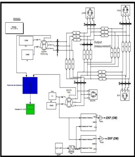
5T. All variables/sizes are given in p.u).Fig 2. Proposed Simulink Diagram.
In this diagram, for the implementation of EKF with OM and DM we use the Embedded MATLAB Function.
First, we consider this values of
Q
k andR
k(Standard version of E.K.F):. . 5
8 . .
9.753*10
0.055664
E K Fk
E K E k
Q
I
R
[image:6.595.322.557.275.446.2]Second, we present the evolution of the estimated output (Pˆ2,3) given by Fig. 3.
Fig 3. Evolution of Pˆ2,3 with OM and DM.
Fig. 3 shows that the OM presents a large variation and don't converge exactly to the real one (error of
10%
). However, with the proposed DM the estimated outputs converge to the real one without error (small error
1%
).Third, we make the following variations in generators parameters (all values are in p.u):
Increase of Internal voltage in generator 1 (E1) from 1.08858 to 1.52 at 12.7ms.
Increase of Input mechanical power at generator 2 (
2 M
P
) from 0.4 to 1.2 at 15.5ms. Increase of Input mechanical power at generator 1 (
1 M
P
) from 1.378644 to 2 between 50ms and 58ms. Decrease of Internal voltage in generator 2 (E2) from 1.65428 to 1 at 72ms.
and we present in Fig. 4 the evolution of error estimation:
Fig 4. Evolution of error estimation with OM and DM. It is clear, according to Fig. 4 that the error estimation converges to 0 (with a small error). While noting that with the DM, the variation is more stable because the elimination of the added elements PV and
Q
with OM which present a large value at the time of variation of generators parameters (could lead the system to diverge).Now, we present the evolution of the norm of error estimation by OM and DM, with the previous values of
Q
kand
R
k or Standard E.K.F (S-E.K.F)) in Fig. 5 and these new values or Modified E.K.F (M-E.K.F) with the proposed choice given by (22) in Fig. 6:. . 3
8 8
. . 3
100
10
10
10
E K F T
k k k
E K E T
k k k k
Q
e e I
I
R
H P H
51.050 51.1 51.15 51.2 51.25
5 10 15 20
time (ms)
E
v
o
lu
ti
o
n
o
f
e
s
ti
m
a
te
d
o
u
tp
u
t
real value OM DM
51.116 51.118 51.12 51.122 51.124
14 16 18
0 10 20 30 40 50 60 70 80
-10 -5 0 5 10 15 20
Time (ms)
E
rr
o
r
E
s
ti
m
a
ti
o
n
Fig 5. Evolution of error estimation with S-E.K.F.
Fig 6. Evolution of error estimation with M-E.K.F. Concerning the evolution of error estimation, the results show that the appropriate choice of matrices
Q
k andR
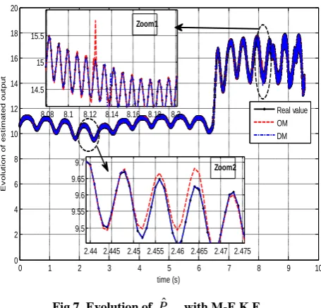
k given by (22) insures the convergence of the estimated states to the real value. Indeed, this is verified by the reduced interval of variation offered by the DM (between -1 and 0.2 with S-E.K.F and between 0.01 and -0.03 with M-E.K.F), however, with OM is between -1.52 and 0.4 with S-E.K.F and 0.06 and -0.05 with the modified version. [image:7.595.49.282.84.276.2]Now, we present the evolution of estimated output with an increase (value equal to three times the nominal) of internal voltage E1 at generator node 1 (with OM and DM):
Fig 7. Evolution of Pˆ2,3 with M-E.K.F.
The result in Fig. 7 shows that the estimated output converges to the real one with a major advantage of the proposed DM in term of stability (without important variation and no increase in value or large peaks).
5.
CONCLUSION
An efficient decoupled dynamic power system model has been described and investigated while based on introducing a transformation of ordinary DAE model using decoupled algorithm. We also used the classical method of E.K.F to real time dynamic state estimation of power systems while including some numerical approximation for the calculation of the Jacobian and which was preceded by a convergence analysis. The results show well the appropriate choice of the dynamic DM in terms of robustness, speed and computing time and, in a very clear way, the high quality of estimation offered by the Modified EKF.
The remaining open questions are the experimental test of the proposed method to large scale power test systems (IEEE 118 bus test system for example).
6.
REFERENCES
[1] Shivakumar N. R. and Amit. 2008. A Review of Power System Dynamic State Estimation Techniques. In Power Syst. Technology and IEEE Power India Conf., India. 1–6.
[2] Neela R. and Aravindhababu P. 2009. A new decoupling strategy for power system state estimation. Int. J. of Energy Convers. and Management. 50. 2047–2051. [3] Thabet A. et al. 2010. Power Systems Load Flow and
State Estimation: Modified Methods and Evaluation of Stability and Speeds Computing. Int. Rev. of Electr. Eng., 5, 1110–1118.
[4] Scholtz E. 2004. Observer based monitors and distributed wave controllers for electromechanical disturbances in power systems. Doctoral Thesis, Massachusetts Institute Technology, USA.
2 4 6 8 10 12 14
-0.4 -0.3 -0.2 -0.1 0 0.1 0.2 0.3 0.4 0.5
Time (ms)
E
rr
o
r
E
s
ti
m
a
ti
o
n
OM DM
0 1 2 3 4 5 6 7 8 9 10
0 2 4 6 8 10 12 14 16 18 20
time (s)
E
v
o
lu
ti
o
n
o
f
e
s
ti
m
a
te
d
o
u
tp
u
t
2.44 2.445 2.45 2.455 2.46 2.465 2.47 2.475 9.5
9.55 9.6 9.65 9.7
Real value OM DM 8.08 8.1 8.12 8.14 8.16 8.18 8.2
14.5 15 15.5
Zoom1
Zoom2
2 4 6 8 10 12 14
-1.5 -1 -0.5 0 0.5
Time (ms)
E
rr
o
r
E
s
ti
m
a
ti
o
n
[image:7.595.51.282.326.513.2][5] Pai M.A., Sauer P.W., Lesieutre B.C and Adapa R. 1995. Structural stability in power systems effect of load models. IEEE Trans. on Power Syst.10, 609–615. [6] Dafis C.J. 2005. An observbility formulation for nonlinear
power systems modeled as differential algebraic systems. Doctoral Thesis, Drexel university, PA, USA.
[7] Debes A.S. and Larson R.E. 1970. A dynamic estimator for tracking the state of a power system. IEEE Trans .on Power App. And Syst. 89, 1670–1678.
[8] Aslund J. and Frisk F. 2006. An observer for nonlinear differential-algebraic systems. Autmatica. 42, 959–965. [9] Wichmann T. 2001. Simplification of nonlinear DAE
systems with index tacking. In European Conf. on Circuit Theory and Design, Espoo, Finland, 173–176. [10] Nikoukhah R., Willsky A. and Levy B. 1992. Kalman
filtering and riccati equations for descriptor systems. IEEE Trans. on Autom. Control. 37, 1325–1342. [11] Isabel M.F. and Barbosa F.P. 1994. Square root filter
algorithm for dynamic state estimation of electric power systems. In Electrotechnical Conference, 7th Mediterranean, Antalya, Turkey, 877–880.
[12] Shih K. and Huang S. 2002. Application of a robust algorithm for dynamic state estimation of a power system. IEEE Trans. on Power Syst. 17, 141–147. [13] Yu K., Watson N. and Arrillaga J. 2005. An adaptive
kalman filter for dynamic harmonic state estimation and harmonic injection tracking. IEEE Trans. on Power Delivery. 20, 1577–1584.
[14] Ma H. and Grigis A. 1996. Identification and tracking of harmonic sources in a power system using kalman filter. IEEE Trans. on Power Delivery. 11, 1659–1665. [15] Beids H. and Heydt G. 1991. Dynamic state estimation
of power system harmonic using kalman filter methodology. IEEE Trans. on Power Delivery. .6, 1663– 1670.
[16] Chowdhury F., Christensen J. and Aravena J. 1991. Power system fault detection and state estimation using
kalman filter with hypothesis testing. IEEE Trans. on Power Delivery. 6, 1025–1030.
[17] Roytelman I. and Shahidehpour S. 1993. State estimation for electric power distribution systems in quasi real-time conditions. IEEE Trans. on Power Delivery. 8, 2009–2015.
[18] Gordon B.W. 2003. Dynamic sliding manifolds for realization of high index differential-algebraic systems. Asian J. of Control., 5, 454–466.
[19] Tarraf D.C. and Asada H.H. 2002. On the nature and stability of differential-algebraic systems. In Proc. American Control Conf., Anchorage, Al USA, 3546– 3551.
[20] Eremia M., Trecat J. and Germond A. 2000. Réseau électriques: Aspects Actuels, 2nd ed. Bucuresti: EdituraTehnica.
[21] Karlsson D. and Hill D.J. 1994. Modelling and identification of nonlinear dynamic loads in power systems. IEEE Trans. on Power Syst. 9, 157–166. [22] Judd K. 2003. Nonlinear state estimation
,indistinguishable states and the extended kalman filter. Physica D: Nonlinear Phenomena. 183, 273–281. [23] Becerra V.M., Roberts P.D. and Griffiths G.W. 2001.
Applying the extended kalman filter to systems described by nonlinear differential-algebraic equations. Control Eng. Practice. 9, 267–281.
[24] Boutayeb M. and Aubry C. 1999. A strong tracking extended kalman observer for nonlinear discrete-time systems. IEEE Trans. on Autom. Control. 44, 1550– 1556.
[25] Boutayeb M. 2000. Identification of nonlinear systems in the presence of unknown but bounded disturbances. IEEE Trans. on Autom. Control. 45, 1503–1507. [26] Song Y. and Grizzle J. 1995. The extended kalman