Local Contrast Enhancement using Local Standard
Deviation
S. Somorjeet Singh
Th. Tangkeshwar Singh
Department of Computer Science
Asst. Prof. (Sr. Scale), Dept. of Computer Science
Manipur University, Canchipur
Manipur University, Canchipur
H. Mamata Devi, PhD.
Tejmani Sinam
Assoc. Prof., Dept. of Computer Science
Assoc. Prof., Dept. of Computer Science
Manipur University, Canchipur
Manipur University, Canchipur
ABSTRACT
For a detailed visibility of an image, since only the global enhancement is not sufficient, local contrast enhancement plays a great role. One of the successful locally adaptive image contrast enhancement methods is by using Local Standard Deviation (LSD). The contrast enhancement using LSD is successfully used in many applications like in medical images, real time images, surveillance applications and many others. These types of applications employ a contrast factor which is divided by LSD. For such type of methods, limitation occurs when the LSD becomes zero. This limitation due to divide by zero can be overcome by adjusting the LSD to a modified value.
Keywords
Local contrast enhancement, local standard deviation, divide-by-zero, removal.
1. INTRODUCTION
People love good quality pictures or images. However, all the pictures or images are not always having good quality depending on various factors like recording, recording device, light incident on the objects and processing etc. One of the low quality images is the low contrast image type. Low contrast images are having narrow range of intensity levels of the pixels of the image. To improve the visual quality of low contrast images, different enhancement can be done in different domain like spatial domain, frequency domain etc.
Global contrast enhancement techniques [1]-[5] work fine, fast and simple for some kind of images. It improves the quality of the image globally, however, the quality of the local contrast is poor in some images. One of the widely utilized global enhancement methods is histogram equalization. Global Histogram Equalization (GHE) is very effective and the most appropriate enhancement method for some images. However, GHE is not always desirable [6], because it produces the image over enhanced in some portions and some properties of the image cannot be defined properly.
Since the image characteristics differ considerably from one region to another in the same image, the enhancement techniques based on local contrast are necessary. There are several local contrast enhancement methods. Dorst [7] adapted histogram stretching method over a neighbourhood around the candidate pixel for local contrast stretching, and followed by a numerous modifications [8]-[10] of histogram equalization based on adapting the same over a sub-region of the image. A local contrast stretching method as suggested by Lee [11],[12]
makes use of local statistics of a predefined neighbourhood in modifying the gray level of a pixel. Narendra and Fitch [13] designed the amplification factor too to be a function of the pixel based on the local gray level statistics over the same neighbourhood in which contrast gain is inversely proportional to LSD.
Dah-Chung [14] observed that image enhancement with contrast gain which is constant or inversely proportional to the LSD produces either ringing artifacts or noise over enhancement due to the use of too large contrast gains in regions with high and low activities, and developed a new method in which gain is a non-linear function of LSD and observed that this method is effective for medical images. Schutte [15] introduced a multi-window extension of this technique and showed how the window sizes should be chosen. Sascha [16] implemented an improved multi-window real-time high frequency enhancement scheme based on LSD in which gain is a non-linear function of the detail energy and observed that this method is effective for the surveillance and many other applications.
The local contrast enhancement using LSD is powerful in many applications. However, for some kind of images, the pixels of some regions of the image are producing the LSD’s as 0’s. This is an undesired limitation that divide by zero may not be working or may produce undesired output image.
This paper is organized as follows: Section 2 briefly reviews some methods based on LSD. Section 3 describes our proposed technique on removal of divide by zero. Section 4 shows experimental results and discussion. And Section 5 is for conclusion.
2. REVIEW
ON
SOME
METHODS
BASED
ON
LOCAL
STANDARD
DEVIATION
In this section, we review some methods in which LSD’s are employed.
First, one of the most frequently referred methods is Narendra and Fitch’s [13] method. They presented a method using LSD information as
( , )
( , )
( , )
( , )
( , )
x x
x
D
f i j
m i j
x i j
m i j
i j
where x(i,j) is the gray scale value of a pixel in an image, f(i,j)
is the enhanced value of x(i,j), mx(i,j) is the local mean, x(i,j)
is the LSD and D is a constant. Here, contrast gain itself is spatially adaptive and inversely proportional to LSD.
Next is also one of the most frequently referred methods. Dah-Chung [14] presented another method using LSD information as
( , )
( , )
( , )
( , )
( , )
( , )
x x xx i j
m i j
f i j
m i j
k i j
i j
(2)where k(i,j) is the contrast gain. This was applied on medical images.
Next is the Multi-Scale Adaptive Gain Control method of Schutte [15]. He described the enhanced output image as
1
(
)
k j j j jC
o
i
M
i
m
LSD
(3)where, o is the output image, i is the input image, k is the number of scales used, M is the global mean of the image, mj is
the local mean of the kernel, Cj is the gain factor that control the
enhancement level per kernel and LSDj is the local standard
deviation per kernel.
Sascha [16] presented another improved method in which frequency bands are separately controlled and enhanced. This is achieved by subtracting windows of two subsequent scales so that the difference between windows represents a supplementary frequency band which is added to a certain pixel neighbourhood and which is additionally enhanced by the use of the bigger kernel:
1 1
(
)
k j j j j jC
o
i
M
m
m
LSD
(4)In all of the methods, (1)-(4), there employed a factor which is divided by the LSD. They are applied for different fields like medical images, real-time imaging, surveillance applications and many other applications. However, they may not be working or may produce undesired output image for some images in which LSD’s of some pixels of the image are zero.
3. REMOVAL OF DIVIDE BY ZERO
CONDITION
In the above equations (1)-(4), if LSD’s of some of the pixels of the image are having the value zero, divide by zero is occurred. This divide by zero can be removed by increasing the window size or by modifying the values of LSD’s of the image.
Although we can verify the removal of divide by zero condition in any of the above equations (1)-(4) or any similar equations, let us take the following method, for the simplicity, for verification:
( , )
( , )
( , )
( , )
( , )
C
f i j
x i j
x i j
m i j
i j
(5)where, x(i,j) is the gray scale value of a pixel in an image, f(i,j)
is the enhanced value of x(i,j), m(i,j) is the local mean, (i,j) is the LSD and C is a constant for contrast control.
Now, the two alternative techniques can be considered for the removal of divide by zero condition. First, it can be removed by increasing the size of the window because LSD’s are zero when all the gray scale values of the pixels under the window are equal.
If the size of the window is taken larger, the chances for the gray scale values of the pixels under the window to be equal are less.
Secondly, each of LSD can be modified by adding a very small value which is greater than zero and a negligible value too. Now, equation (5) can be improved as
( , )
( , )
( , )
( , )
( , )
C
f i j
x i j
x i j
m i j
i j
s
(6) [image:2.595.309.552.395.632.2]where, s is a very small and negligible quantity greater than zero. When s is very small, equation (6) maintains the same quality of equation (5) except it removes the divide by zero condition for an output image. Human perception is no difference between the output images produced by the equations (5) and (6) of the same input image, except the divide by zero portions of the image, because human eye cannot detect the difference at the micro level or lower level for any intensity value of a pixel.
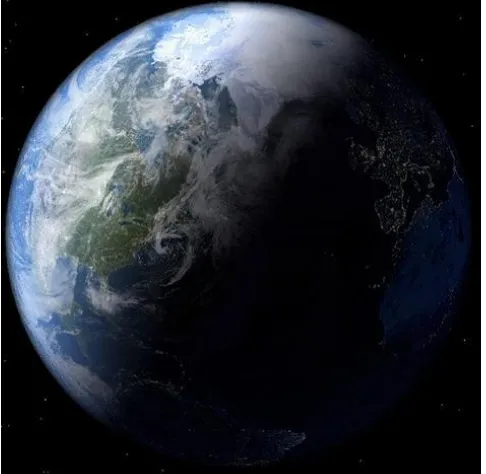
Fig. 1. Photograph of earth from space
window for the second method i.e., equation (6). Hence, the second technique is the better method.
4. EXPERIMENTAL
RESULT
AND
[image:3.595.311.545.71.211.2]DISCUSSION
Table 1. No. of LSD with zero values against the window size
Size of Window
(One side each) No. of LSD with 0 value
3 62275
5 49898
7 39707
9 35159
11 34038
13 30648
15 27517
17 24771
19 22712
21 20783
23 18898
25 17121
27 15519
29 14017
31 12568
35 10106
55 3765
75 1659
85 1133
95 732
105 397
115 133
117 90
119 49
121 15
123 0
125 0
We have tested the above two techniques for the removal of divide by zero condition in MATLAB 7.13.0.564 with different window sizes. A detailed study is performed on a satellite image, i.e., the photograph of earth taken from the space as in
Fig. 1. First, we have counted the number of LSD’s having the
[image:3.595.57.302.134.611.2]value zero against the relevant window sizes. Table 1 shows the relevant information with different window sizes. When the size of the window is small, number of LSD’s with zero value is larger. If the size of the window is increased, the number of LSD’s with zero value is smaller.
Fig. 2. Graph showing No. of LSD’s with zero values against the Size of Window
(a) With window size 25x25 (b) With window size 35x35
(c) With window size 55x55 (d) With window size 85x85
(e) With window size 95x95 (f) With window size 125x125
Fig.3. Test images with different window sizes using eqn. (5)
When the size of the window is equal to 123x123 or greater than 123x123, there is no LSD with the value zero. The relation between the size of the window and the number of LSD’s with zero values is illustrated in the graph as shown in Fig. 2. Next, we have applied the equation (5) with different window sizes on the image, shown in Fig. 1, by taking the same C value.
[image:3.595.306.551.241.639.2]divide by zero condition, are shown. When the window size is increased, the size of undesired effect due to divide by zero is reduced. And no undesired effect due to divide by zero found when window size is 125x125. However, the enhancement quality is reduced in increasing the window size too much. The first technique is, therefore, limited to the nature of the image.
(a) With equation (5), Window size=25x25
(b) With eqn. (6), s=1.0x10⁻¹², Window size=25x25
(c) With equation (5), Window size=55x55
[image:4.595.53.296.144.430.2](d) With eqn. (6), s=1.0x10⁻¹², Window size=55x55
Fig.4. Comparative Results with C=0.1 (Using HSI format)
Table 2. Comparative Statements of Our Proposed Technique with Other Methods
Methods of Equations (1)-(4)
With Our Proposed Technique
If the LSD’s of the pixels are zero, undesired similar effect due to divide by zero conditions are produced with these methods as shown in fig.
3(a)-(e), fig. 4(a) and fig. 4(c).
No such undesired effect due to divide by zero conditions
are produced. To control the undesired effect due to
divide by zero conditions, the size of the window is to be increased up to a certain amount, however, it may reduce
the quality of the enhancement
Any desired size of the window can be taken without any undesired effect due
to divide by zero conditions. When we examined with the second method, i.e., equation (6), any size of window can be taken as our desire. If we desire the window size to be 25x25, a comparison for equations (5) and (6) is shown in Fig. 4 (a) and (b). If we desirethe window size to be 55x55, the difference of equations (5) and (6) is shown in
Fig. 4 (c) and (d). Here, the value of C is taken as 0.1 and the value of s for equation (6) is taken as 0.000000000001, i.e., 1.0x10⁻¹² which is a negligible quantity. From these experiments, we have found that there is no difference between the quality in the enhancement of equations (5) and (6), except the divide by zero portions in the image. This means that divide by zero can be overcome easily with the technique of equation (6) at any desired level of window size.
The distinctive features of the proposed technique are shown in the comparative statements with equations (1)-(4), given in the
Table 2.
5. CONCLUSION
Local Contrast Enhancement using LSD is widely used in different fields like Medical imaging, Real-Time Imaging, Surveillance and Security Applications and many others. Many people working with LSD for Local Contrast Enhancement may be suffering from divide by zero. This paper presents the removal techniques of the divide by zero effect without changing the enhancement quality. This paper will be beneficial to all who are interested on Local Contrast Enhancement using LSD.
6. REFERENCES
[1] S. Somorjeet Singh, Dr. H. Mamata Devi, Th. Tangkeshwar Singh, O. Imocha Singh, “A New Easy Method of Enhancement of Low Contrast Image Using Spatial Domain,” International Journal of Computer Applications (0975 – 8887) Volume 40– No.1, February 2012
[2] R. C. Gonzalez and R. E. Woods, Digital Image Processing. 3rd edition, Prentice Hall, 2008.
[3] Sascha D. Cvetkovic and Peter H. N. de With, "Image enhancement circuit using non-linear processing curve and constrained histogram range equalization," Proc. of SPIE-IS&T Electronic Imaging, Vol. 5308, pp. 1106-1116 (2004).
[4] M.A. Yousuf, M.R.H. Rakib, “An Effective Image Contrast Enhancement Method Using Global Histogram Equalization,”Journal of Scientific Research, Vol. 3, No. 1, 2011.
[5] I. Altas, J. Louis, and J. Belward, “A variational approach to the radiometric enhancement of digital imagery,” IEEE Trans. Image Processing, vol. 4, pp. 845–849, June 1995. [6] T.-L. Ji, M. K. Sundareshan, and H. Roehrig, “Adaptive
image contrast enhancement based on human visual properties,” IEEE trans. Med. Imag., vol. 13, pp. 573–586, Aug. 1994.
[7] L. Dorst, “A local contrast enhancement filter,” In Proc. 6th Int. Conference on Pattern recognition, pages 604-606, Munich, Germany, 1982.
[8] D. Mukherjee and B. N. Chatterji, “Adaptive neighborhood extended contrast enhancement and its modification,” Graphical Models and Image Processing, 57:254-265, 1995.
[9] R. B. Paranjape, W. M. Morrow, and R. M. Rangayyan, “Adaptive-neighborhood histogram equalization for image enhancement,” Graphical Models and Image Processing, 54:259-267, 1992.
[10] S. M. Pizer, E. P. Amburn, J. D. Austin, R. Cromartie, A. Geselowitz, T. Geer, B. H. Romeny, J. B. Zimmerman, and K. Zuiderveld, “Adaptive histogram modification and its variation,” Computer Vision, Graphics and Image Processing, 39:355-368, 1987.
[12] J. S. Lee, “Refined filtering of image noise using local statistics,” Computer Graphics and Image Processing, 15:380-, 1981.
[13] P.M. Narendra and R.C. Fitch, "Real-time adaptive contrast enhancement," IEEE Trans. PAMI, Vol.3, no. 6, pp.655-661, 1981.
[14] D.-C. Chang and W.-R. Wu, "Image contrast enhancement based on a histogram transformation of local standard
deviation," IEEE Trans. MI, vol. 17, no. 4, pp. 518-531, Aug. 1998.
[15] K. Schutte, "Multi-Scale Adaptive Gain Control of IR Images," Infrared Technology and Applications XXIII, Proceedings of SPIE Vol. 3061, pp.906-914 (1997). [16] Sascha D. Cvetkovic, Johan Schirris and Peter H. N. de