Application of Fuzzy Controlled TCSC in Multi Machine
Power system for Transient Stability Improvement
K.Srinivas
Assistant Professor JNTUH College of Engineering
Karimnagar, AP, India.
ABSTRACT
For the improvement of transient stability the general methods adopted are fast acting exciters, circuit breakers and reduction in system transfer reactance. The modern trend is to employ FACTS devices in the existing system for effective utilization of existing transmission resources. These FACTS devices contribute to power flow improvement besides they extend their services in transient stability improvement as well in this paper, the work had been carried out in order to improve the Transient Stability of WSCC 9 Bus System with Fixed Compensation on Various Lines and Optimal Location has been investigated using trajectory sensitivity analysis for better results. In order to improve the Transient Stability margin further series FACTS device has been implemented. A fuzzy controlled Thyristor Controlled Series Compensation (TCSC) device has been used here and the results highlight the effectiveness of the application of a TCSC in improving the transient stability of a power system.
Keywords
Fuzzy Logic, FACTS, Power system Stability
1.
INTRODUCTION
Power system stability has been recognized as an important problem for secure system operation since the 1920s. Many major blackouts caused by power system instability have illustrated the importance of this phenomenon. As power systems have evolved through continuing growth in interconnections, use of new technologies and controls, and the increased operation in highly stressed conditions, different forms of system instability have emerged. For example, voltage stability, frequency stability and inter area oscillations have become greater concerns than in the past. This has created a need to review the definition and classification of power system stability. A clear understanding of different types of instability and how they are interrelated is essential for the satisfactory design and operation of power systems. Power system stability is the ability of an electric power system, for a given initial operating condition, to regain a state of operating equilibrium after being subjected to a physical disturbance, with most system variables bounded so that practically the entire system remains intact [1].The power system is a highly nonlinear system that operates in a constantly changing environment; loads, generator outputs and key operating parameters change continually. When subjected to a disturbance, the stability of the system depends on the initial operating condition as well as the nature of the disturbance. Stability of an electric power system is thus a property of the system motion around an equilibrium set, i.e., the initial operating condition. In an equilibrium set, the various opposing forces that exist in the system are equal instantaneously or over a cycle.Power systems are subjected to a wide range of disturbances, small and large. Small
2.
TRAJECTORY
SENSITIVITY
ANALYSIS
1.1 Computation of Trajectory Sensitivity
Multi machine power system [4] [5] [6] is represented by a set
of differential equations
( , , ),
(
0
)
0
x
f t x
x t
x
(3.1)Where x is a state vector and
is a vector of system parameters. The sensitivities of state trajectories with respect to system parameters can be found by perturbing
from itsnominal value
0 .The equations of trajectory sensitivitycan be found
as[6]
x
f
x
f
,
x
(
t
o
)
0
x
(3.2)Where
x
x
/
. Solution of (3.1) and (3.2) gives the state trajectory and trajectory sensitivity, respectively. However sensitivities can also be found in a simpler way by using numerical method.1.2 Numerical Evaluation
To explain this method, let us choose only one parameter, i.e.,
becomes a scalar and the sensitivities with respect to it are studied. Two values of
are chosen (say
1and
2). The corresponding state vectors x1 and x2 respectively are thencomputed. Now the sensitivity at
1 is definedas
2
1
2
1
x
x
x
Sens
(3.3)If
is small, the numerical sensitivity is expected to be very close to the analytically calculated trajectory sensitivity. In the case of power system, sensitivity of state variables, e.g., the generator rotor angle (
) and per unit speed deviation(
r) can be computed as in (3.3) with respect to someparameter
. Now one of the generators, say the jth one, is taken as the reference. Then, the relative rotor angle of the ithmachine (i.e. the excursion of
ij with respect to the rotorangle of reference machine) is given by
ij
i
j. Thesensitivity of
ij with respect to
is computed asij i j
(3.4)
1.3 Quantification of TS and Its Implication
Trajectory sensitivities (
ij/
and
ri/
) give us information about the effect of change of parameter on individual state variables and hence on the generators (to which the particular state variable correspond) of the system. However to know the overall system condition, we need to sum up all these information. The norm of the sensitivities ofij
and
ri are calculated for this. The sensitivity normfor an m machine system is given as
2 2
1
m ij ri
S N i
(3.5)
A new tem
(ETA) is introduced.
Is defined as theinverse of the maximum of SN , i.e .,
1
/
max(
S
N)
. Asthe system moves towards instability, the oscillation in TS will be more resulting in larger values of SN. This will result in the smaller values of η. Ideally η should be zero at the point of instability. Therefore the value of η gives us an indication of distance from instability. In this paper η is used for assessing the relative stability conditions of the system with different values of fault clearing time, system load and firing angle of TCSC.
Consider a fault in one of the lines of the system. The post-fault conditions are studied by continuously increasing the fault clearing time (tcl). The system states will oscillate more and take longer time to settle as tcl is increased. The sensitivities of the state variables will also exhibit large oscillations for increasing tcl. These oscillations will become unbounded as tcl exceeds the critical clearing time. Thus large peaks in trajectory sensitivity (TS) clearly indicate the proximity of the parameter to the critical value beyond which the system becomes unstable.
The sensitivity of relative rotor angle is considered here instead of the sensitivity of
of an individual machine because the relative rotor angle is the relevant factor when angular stability is concerned.3.
THYRISTOR-CONTROLLED SERIES
CAPACITOR (TCSC)
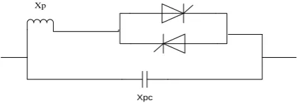
The basic Thyristor-Controlled Series Capacitor scheme, proposed in 1986 by Vithayathil with others [2] [3] as a method of “rapid adjustment of network impedance,” is shown in the fig.3.1.It consists of the series compensating capacitor shunted by a Thyristor-Controlled Reactor. In a practical TCSC implementation, several such basic compensators may be connected in series to obtain the desired voltage rating and operating characteristics.
Xp
[image:2.595.323.536.542.616.2]Xpc
Fig 3.1 Equivalent circuit of TCSC
This arrangement is similar in structure to the TSSC and, if the impedance of the reactor, XL, is sufficiently smaller than
that of the capacitor, Xc, it can be operated in an on/off manner like the TSSC. However, the basic idea behind the TCSC scheme is to provide a continuously variable capacitor by means of partially canceling the effective compensating capacitance by the TCR.
impedance, Xc, and a variable inductive impedance, XL (α),
that is,
XTCSC(α) = (Xc*XL)/(XL(α)-Xc)
Where XL(α)=XL*π / (π-2 α-sin α), XL≤XL(α )≤∞
XL = ωL, and α is the delay angle measured from the crest of
the capacitor voltage.
The [7] TCSC thus presents a tunable parallel LC circuit to the line current that is substantially a constant alternating current source. As the impedance of the controlled reactor, XL(α), is varied from its maximum (infinity) toward its
minimum(ωL), the TCSC increases its minimum capacitive impedance, XTCSCmin =Xc=1/ωC,(and thereby the degree of
series capacitive compensation) until parallel resonance at Xc=XL(α) is established and XTCSCmax theoretically becomes
infinite. Decreasing XL(α) further, the impedance of the
TCSC, XTCSC(α) becomes inductive, reaching its minimum
value of XLXc/(XL-Xc) at α=0, where the capacitor is in effect
bypassed by the TCR. Therefore, with the usual TCSC arrangement in which the impedance of the TCR reactor, XL,
is smaller than that of the capacitor, Xc, the TCSC has two operating ranges around its internal circuit resonance: one is the αclim≤ α≤л/2 range, where XTCSC(α) is capacitive, and the
other is the 0≤ α≤ αLlim range, where XTCSC(α) is inductive.
The steady state model of the TCSC described above is based on the characteristics of the TCR established in an SVC environment, where the TCR is supplied from a constant voltage source. This model is useful to maintain a basic understanding of the functional behavior of the TCSC. However, in the TCSC scheme the TCR is connected in shunt with a capacitor, instead of a fixed voltage source. The dynamic interaction between the capacitor and the reactor changes the operating voltage from that of the basic sine wave established by the constant line current. Refer to the basic TCSC circuit shown in above figure. Assume that the thyristor valve, sw, is initially open and the prevailing line current I produces voltage Vco across the fixed series compensating capacitor. Suppose that the TCR is to be turned on at α measured from the negative peak of the capacitor voltage. As seen, at this instant of turn-on, the capacitor voltage is negative; the line current is positive and thus charging the capacitor in the positive direction. During this first half-cycle of TCR operation, the thyristor valve can be viewed as an ideal switch, closing at α, in series with a diode of appropriate polarity to stop the conduction as the current crosses zero.
4.
MODELING OF TCSC AND THE
POWER SYSTEM
The TCSC model is given in Fig. 4.4. The overall reactance XC of the TCSC is given in terms of the firing angle α as [6] [8]:
( ) 5
1 2 4
XC XFC XFC Where
2( ) sin( )
1
,
2 XFC PXXFC XP
, tan[ ( )] tan( )
3 X FCX P 4 3 3
2 2
4 2cos ( )
5 X P
Let us denote the fundamental frequency capacitance of the TCSC, which is equal to 1/(ωsXC), as Ctcsc. It is to be noted
That in this work the TCSC is operated only in the capacitive mode. The capacitive reactance XFC of the TCSC is chosen as half of the reactance of the line in which the TCSC is placed and the TCR reactance XP is chosen to be 1/3 of XFC.
The system studied in this paper is the WSCC 3 machine nine-bus system shown in Appendix. A three-phase fault is simulated in one of the lines of the nine-bus system. The simulation is done in three steps. To start with, the pre-fault system is run for a small time. Then, a symmetrical fault is applied at one end of a line. Simulation of the faulted condition continues till the fault is cleared after a time tcl. Then, the post-fault system is simulated for a longer time (say 5 s) to observe the nature of the transients. The fault may be of self-clearing type (i.e. isolation of line is not required for fault clearance) or may be cleared by isolating the faulted line
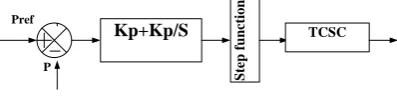
1.4
The Control Scheme
In the next step, a controller is employed along with the TCSC
[9] [10]. The block diagram of the control scheme used is
shown in Fig.4.1.
Kp+Kp/S
S
te
p
f
u
n
ct
io
n
TCSC
[image:3.595.321.520.380.431.2]P Pref
Fig. 4.1 PI Control Scheme of TCSC
The active power flow (P) through the line containing TCSC is taken as the control variable. It is compared with the reference value of active power flow (Pref) and the error is fed to a PI controller. The output of the PI is the firing angle of the TCSC, α. This α is passed through a limiter to keep it within the capacitive operation zone of the TCSC (between 145◦ and 180◦). The output of the limiter is supplied to the firing circuit of TCSC. The capacitance value of the TCSC (Ctcsc) is computed as described in Modeling Section. This capacitance is then included in the line dynamics. This scheme is sufficient if the fault is only of self-clearing type, because there is no change in system configuration and hence the steady state power flow should remain the same before and after the fault. But when isolating the faulty line clears the fault, the system configuration changes resulting in a change of the steady state power flow through the lines, Therefore, a corresponding change in Pref is needed.
The effect of the TCSC on the transient stability of the system depends largely on the proper functioning of the controller. Therefore, choice of suitable values of controller constants KP and KI is very important.
TCSC causes improvement of system stability condition the most when it is placed in line 6–9 or line 5–7. So, henceforth we shall study the effect of TCSC (along with controller) in these two locations.
loop, i.e., without a controller. In open loop, the TCSC acts as a fixed capacitor throughout the period of disturbance. Let us term this as the fixed capacitor mode of operation. The effects of this fixed capacitor and the effects of a TCSC-controller combination (with suitably chosen controller constants) on the transient stability condition are investigated and compared here.
Therefore, it can be concluded that the improvement in the transient stability condition of the system is much more with the TCSC-controller combination. These results highlight the effectiveness of the application of a TCSC along with a controller in improving the transient stability of a power system.
5.
FUZZY LOGIC CONTROLLER
Fuzzy modeling is the method of describing the characteristics of a system using fuzzy inference rules. The method has a distinguishing feature in that it can express linguistically complex non-linear system. It is however, very hand to identify the rules and tune the membership functions of the reasoning. Fuzzy Controllers are normally built with fuzzy rules. These fuzzy rules are obtained either from domain experts or by observing the people who are currently doing the control. The membership functions for the fuzzy sets will be derive from the information available from the domain experts and/or observed control actions. The building of such rules and membership functions require tuning. That is, performance of the controller must be measured and the membership functions and rules adjusted based upon the performance. This process will be time consuming.
The basic configuration of Fuzzy logic control based as shown in Fig. 5.1 consists of four main parts i.e.
(i) Fuzzification, (ii) knowledge base, (iii) Inference Engine and (iv) Defuzzification
Data Bus
Controlled System
Interface Engine Defuzzifier Fuzzifier
[image:4.595.54.279.474.586.2]Rule base and Knowledge base
Fig. 5.1 Structure of Fuzzy Logic controller
1.5 Algorithm
(a) Initial compensation of (30-50%) is provided in the line where Tcsc is to be placed by reducing the line reactance and change ybus in the following steps.
(i) All system data are converted to a common base; a system base of 100MVA is frequently used. Form Ybus and run load flow
(ii) The mechanical power input is taken as (Pm = Pinj ) of the
generators.
(iii)The loads are converted to equivalent impedances or admittances. The needed data for this step are obtained from the load flow study. Thus if a certain load bus has a voltage
VL, power PL, reactive power QL, and current IL flowing into a
load admittance YL=GL+j BL, then
PL+j QL=VL IL* = VL {VL*(GL-jBL)} =VL2(GL-j BL)
The equivalent shunt admittance at that bus is given by YL=PL / VL
2
– j (QL / VL 2
)
(iv)The internal voltages of the generators Ei∟δi0 are
calculated from the load flow data. These internal angles may be computed from the pretransient terminal voltages V∟α as follows. Let the terminal voltage be used temporarily as a reference. If we define I=I1+j I2 , then from the relation
P+j Q = VI* we have I1+j I2 = (P – j Q)/V,
But since
E∟δ’ = V+jxd’I,
We compute E∟δ’= (V + QXd’/V) + j (PXd’/V
(v) The initial generator angle δ0 is then obtained by adding
the pretransient voltage angle α to δ’, or δ0= δ’+ α
(b) For fault mode:
(i) For faulted mode, find generator outputs from power angle equations and solve swing equations by R.K fourth order method etc.
Voltages at each bus is obtained by v=inv(ytrbus)*Inor
ytrbus(fb,fb)=ytrbus(fb,fb)+complex(0.0,-999999999), where fb is fault bus. For each time step
Solve swing equations using R.K. fourth order and calculate deltas of generators for fuzzy controller take
error(1)=(Pf(ltc)-Pref(ltc)), where ltc=line having tcscdelerr=error(1)-error(0) as inputs and output of Xtcsc gives the compensation to be provided. The line impedance becomes.
zl(ltc)=complex(r(ltc),x(ltc)-Xtcsc),change elements in ytransbus
6.
SIMULATION AND RESULTS
Fig.6.1 Test system: WSCC 9-bus system (Western System Coordinating Council), Anderson Text)
0 0.5 1 1.5 2 2.5
-2 -1 0 1 2 3 4
X: 0.02 Y: -0.6867
time in sec
acti
ve
power flow in p.u
line flows Vs time
[image:5.595.320.539.80.336.2]data1 data2 data3 data4 data5 line6 data7 data8 data9
Fig. 6.2 Power flow in line 6 without compensation
0 0.5 1 1.5 2 2.5
-3 -2 -1 0 1 2 3 4
X: 0.015 Y: -0.9846
time in sec
acti
ve
power flow in p.u
power flow Vs time
data1 data2 data3 data4 data5 line6 data7 data8 data9
Fig. 6.3 Power flow in line 6 with 50% compensation
0 5 10 15 20 -30
-20 -10 0 10 20 30 40 50 60 70
X: 0.72 Y: 65.73
time in sec
del2
1,del
31(i
n degree
s)
Relative Rotor angle Vs time
[image:5.595.57.276.318.463.2]del21 del31
Fig. 6.4 Fixed compensation in line (6-9) fault at bus 5,tcl=0.2s
0 5 10 15 20
-30 -20 -10 0 10 20 30 40 50 60 70
time in sec
del2
1,del
31(i
n degree
s)
Relative Rotor angle Vs time
X: 0.725 Y: 60.27
del21 del31
Fig. 6.5 PI controller in line (6-9) fault at bus 5, tcl=0.2s
0 5 10 15 20
-20 0 20 40
Time in sec
Del21
,Del3
1 (in de
grees
) X: 0.67Y: 35.83 RELATIVE ROTOR ANGLE Vs TIME
0 5 10 15 20
-1 0 1 2 3
Time in sec
Active
power Gene
ration in( P.
U) ACTIVE POWER GENERATION Vs TIME
Pg1 Pg2 Pg3 del21 del31
Fig. 6.6 Fuzzy controller in line 6-9, fault at bus 5 tcl 0.2s
7.
CONCLUSION
In the steady state, FACTS controllers like TCSC help in controlling the power flow through a line. Since power systems are non-linear, conventional controllers PI cannot perform well in maintaining power system stability. When firing angle of TCSC is controlled using conventional PI controller reduction in first swing peak value is observed when compared to fixed compensation. By comparing the above results we can conclude that, with TCSC Controller incorporated in the line 6-9 for a fault at bus 5. This shows the improvement of Transient Stability with FUZZY controller over PI Controller and there is a significant improvement in the Transient Stability with variable series Compensation.
8.
REFERENCES
[image:5.595.316.543.396.546.2] [image:5.595.60.273.499.654.2]Power System Security Assesment”, IEEE Trans. on Power Systems., Vol. 26, No. 4, pp 2319-2327, 2011.
[2] Dheeman Chatterjee, Arindam Ghosh∗, “TCSC control design for transient stability improvement of a multi-machine power system using trajectory sensitivity”, Department of Electrical Engineering, Indian Institute of Technology, Kanpur 208 016, India.
[3] Dheeman Chatterjee , Arindam Ghosh*, “Application of Trajectory Sensitivity for the Evaluation of the Effect of TCSC Placement on Transient Stability” International Journal of Emerging Electric Power Systems, Volume 8, Issue 1 2007 Article 4, The Berkeley Electronics.
[4] Monteiro Pereira, R.M. Machado Ferreira, C.M.Maciel Barbosa, F.P, “Dynamic voltage stability assessment of an electric power system using trajectory sensitivity analysis,” IEEE Power Tech, 2009, pp. 1-6.
[5] Chatterjee, D. and Ghosh, A. “Using Trajectory sensitivity for stability Assessment of a Ward-PV Equipment Power System,” IEEE Power Engineering Society General Meeting: 2007, pp. 1-7.
[6] Nguyen T.B., Dynamic Security Assessment of Power Systems using Trajectory Sensitivity Approach, Dept. of Electrical & Computer Engg, University of Illinois at Urbana-Champaign, 2002.
[7] Nguyen T.B. and Pai M.A., “Dynamic security-constrained rescheduling of power systems using trajectory sensitivities,” IEEE Trans. Power System, 2003, Vol. 18, No. 2, pp. 848-854.
[8] Soman S.A., Nguyen T.B., Pai M.A. and Vaidyanathan Rajani, “Analysis of angle stability problems A transmission protection systems perspective,” IEEE Transactions on Power Delivery, 2004, Vol. 19, No. 3.
[9] Padiyar K.R. and Uma Rao K, “Discrete control of TCSC for stability improvement in power systems,” Proceedings of the 4th IEEE conference on control applications, 28-29 Sep, 1995.
[10]Shubhanga K.N. and Kulkarni A.M., “Determination of effectiveness of transient stability controls using reduced number of trajectory sensitivity computations,” IEEE Trans. Power System, 2004, Vol. 19, No. 1, pp. 473- 482.