http://dx.doi.org/10.4236/ojapps.2015.56026
How to cite this paper: Hou, F.F. and Ai, K.F. (2015) The Empirical Research of Relationship between Consumption and In-come for Chinese Urban Residents. Open Journal of Applied Sciences, 5, 251-258.
http://dx.doi.org/10.4236/ojapps.2015.56026
The Empirical Research of Relationship
between Consumption and Income for
Chinese Urban Residents
Fangfang Hou, Kefeng Ai
College of Science, University of Shanghai for Science and Technology, Shanghai, China Email: qiexff@163.com
Received 11 May 2015; accepted 13 June 2015; published 16 June 2015
Copyright © 2015 by authors and Scientific Research Publishing Inc.
This work is licensed under the Creative Commons Attribution International License (CC BY). http://creativecommons.org/licenses/by/4.0/
Abstract
This paper studied the clustering analysis of panel data, the specification test of panel data model and its parameter estimation. By carrying out clustering analysis on panel data, we finally decided to study the relationship of Chinese urban residents’ eight income levels between consumption and income from 2007 to 2012. Based on analysis of covariance in panel data model, we built the variable coefficient panel data model and then estimated the model parameters. In this work, we can identify the relationship between consumption and income in recent years. According to the estimation results, we drew the conclusion that income disparities have important influence on urban residents’ consumption behavior.
Keywords
Panel Data, Consumption and Income, Clustering Analysis, Analysis of Covariance, Variable Coefficient, Parameter Estimation
1. Introduction
Panel data refer to two-dimensional data which are obtained in time series and cross section at the same time [1], and that means taking multiple cross sections on time series, and selecting the sample observations on cross sec-tions at the same time. With the development of the society, building model only on time series data or cross section data already cannot satisfy the increasingly complex economic problems. In addition, with the develop-ment of computer technology and internet, access to panel data becomes more and more easy.
252
data model is more efficient; second, panel data provide more information, so as to improve the degree of free-dom of the model, reduce the multi-collinearity among the explanatory variables, and eventually improve the accuracy of parameter estimation [2]; third, panel data model is more suitable for complicated economic prob-lems.
Since the 70’s of the last century, a large number of theoretical and empirical analyses of panel data have sprung up [3][4]. The theory of the general panel data model is mature [5]-[8]. Bai [9] summarized setting, sta-tistical test and new progress of panel data model. Many papers discussed the relationship between consumption and income [10]-[12]. But the data are not in recent years. This paper used the panel data in recent years and combined clustering analysis with panel data. So the conclusion is more consistent with the reality.
This paper preprocessed consumption panel data and income panel data of Chinese urban residents’ eight in-come levels from 2002 to 2012, then carried out clustering analysis on the panel data, and finally concluded that the structures of consumption and income were same from 2007 to 2012. By the analysis of covariance for panel data model, eventually we built the variable coefficient panel data model on consumption panel data and income panel data of Chinese urban residents’ eight income levels from 2007 to 2012. Then, we used Eviews 7.0 to es-timate the parameters of the model, and analyzed the results.
2. Methodology
2.1. Clustering Analysis of Panel Data
The panel data xit, 1,i= ,N t; 1,= ,T contains T cross sections. If we use the distance between the cross sections to measure the similarity, then we obtain a T T× similarity matrix, and it is a symmetrical matrix. The similarity matrix is as follows:
12 13 1
23 2 1, 0 0 0 T T T T T T
δ δ δ
δ δ δ − × ts
δ is a dissimilarity degree measure between the t-th cross section and the s-th cross section, which also is a measure of the distance. When the two time sections are very similar, its value is close to zero.
Here are several kinds of commonly used method for measuring distance between cross sections. As shown below:
1) Euclidean Distance: ( )1
(
)
21
N
ts it is
i
x x
δ
=
=
∑
− .2) Squared Euclidean Distance: ( )2
(
)
21
N
ts it is i
x x
δ
=
=
∑
− .3) Minkowski Distance: ( )
1 3 1 p N p
ts it is
i x x δ = = −
∑
. When p = 2, Minkowski distance is the Euclidean distance.4) Manhattan Distance: ( )4
1
N
ts it is i
x x
δ
=
=
∑
− . Manhattan distance is a special case of the Minkowski distancewhen p = 1.
5) Chebyshev Distance: ( )5
1max
ts it is
i N x x
δ
≤ ≤
= − .
The clustering analysis of panel data can divide time sections into several divisions. Building model on one of the division can ignore unobservable time effect, which has important significance on the application. Zhu and Chen [13] studied the clustering analysis of panel data and its application, and focused on the cluster in cross section.
di-253
vide each cross section into a class, then we have a total of T classes; secondly, according to the above distance calculation, we obtain a similarity matrix of panel data, then we merge the nearest two time sections into a class, so we have T−1 classes; again, according to the similarity matrix, we merge the nearest two time sections into a class, so we have T−2 classes; by analogy, we eventually merge all T time series into a class.
2.2. Analysis of Covariance
To build model on panel data, we must first determine the form of the model. General panel data model is as follows:
, 1, , , 1, , . it i it i it
y =α +x β +u i= N t= T (1)
Among them, xit is a 1×K vector, and βi is a K×1 vector, and K is the number of explanatory va-riables. αi is the intercept item, and its value is related to the individual, and it is regarded as the fixed para-meter to estimate here. uit is a random error term, and it is not associated with explanatory variables, and its mean is zero, and its variance is 2
u
σ , and it is independent and identically distributed. The common situation of model (1) is as follows:
1) when αi =α βj, i =βj, model (1) is called the basic model or mixed regression model; 2) when αi ≠α βj, i =βj, model (1) is called the variable intercept model;
3) when αi ≠α βj, i ≠βj, model (1) is called the variable coefficient model.
The common test for determining the model forms is the analysis of covariance, also is called F test. The test contains two main hypotheses:
Hypothesis 1: The slopes are the same, but the intercepts are not the same. The model is:
, 1, , , 1, , .
it i it it
y =α +x β+u i= N t= T (2)
Hypothesis 2: The intercepts and slopes are the same in different cross sections and different time series. The model is:
, 1, , , 1, , .
it it it
y = +α x β+u i= N t= T (3)
According to the method in parameter constraint test, we can construct test statistics for the above two hypo-theses1. Test statistics for hypothesis 1 and hypothesis 2 respectively are:
(
) (
)
(
)
(
) (
)(
)
(
)
2 1 3 1
1 2
1 1
1 1 1
and
1 1
S S N K S S N K
F F
S N T K S N T K
− − − − +
= =
− − − −
Among them, S S1, 2 and S3 respectively are the sums of squared residuals for model (1), (2) and (3) under ordinary least square method.
When hypothesis 1 is correct, F1F
(
N−1)
K N T,(
− −K 1)
. When hypothesis 2 is correct,(
)(
) (
)
2 1 1 , 1
F F N− K+ N T− −K . Obviously, if we accept hypothesis 2, we don’t need to test hypothesis 1, and we should build model (3). If we reject hypothesis 2, we should test hypothesis 1. If we accept hypothesis 1, we should build model (2). If we reject hypothesis 1, we should build model (1).
2.3. The Parameter Estimation of Variable Coefficient Panel Data Model For fixed effect variable coefficient model (1), it can be rewritten as:
, 1, , , 1, , .
i i i i
y =X b +u i= N t= T (4)
Among them,
( ) ( )
1 1 1 2 1 1 1
2 1 2 2 2 2 1 2
1 2
1 1 1 1 1
1 1
, , , .
1
i i i Ki i i
i
i i i Ki i i
i i i i
i
iT T iT iT KiT T K Ki K iT T
y x x x u
y x x x u
y X b u
y x x x u
α α β β β × × + + × × = = = = = 1
254
The matrix form is:
.
Y =XB+U (5)
Among them,
( ) ( )
1 1 1 1
2 2 2 2
1 1 1 1 1
0
, , ,
0
N NT N NT N K N N K N NT
y X b u
y X b u
Y X B U
y × X × + b + × u ×
= = = =
.
Fixed effect variable coefficient model is also called seeming unrelated regression model. The model consid-ers that coefficients don’t change with time for each individual. It is put forward by Zellnerin 1962. The selec-tion of parameter estimaselec-tion method depends on the random disturbance term2. If E u u
( )
i ′ =j 0,i≠ j and( )
2i i i T
E u u′ =σ I , model (4) can be estimated by ordinary least square method, which is the classic method in single equation econometric model. Namely we take each time series as sample, and use ordinary least squares method to estimate bi respectively, or adopt the generalized least square method to estimate B=
(
b b1 2 bN)
′ at the same time. The two kinds of estimation results are consistent. If E u u( )
i ′ ≠j 0,i≠ j, we can use the gene-ralized least square method to estimate B. We write Ω =ij E u u( )
i ′j , then the covariance matrix of U =(
u1 u2 uN)
′ is:11 12 1
21 22 2
1 2
. N
N
N N NN NT NT
V
×
Ω Ω Ω
Ω Ω Ω
=
Ω Ω Ω
So the generalized least square estimation of the parameters is: ˆ
(
1)
1 1GLS
B = X V′ − X − X V Y′ − .
3. The Empirical Research
According to the consumption theory of Keynes, the total consumption is the function of total income. As we all known, there are a stable and interdependent relationship between consumption and income. Namely income is the decisive factor in influencing consumption. We can relate this kind of relationship with regression theory, and build the linear model C= +α βY on consumption and income. Among them, C is the per capita con-sumption expenditure. Y is the per capita disposable income. α is the intercept item. β is the marginal consumption propensity, and its value is between 0 and 1.
With the development of the society, accessing to panel data becomes more and more easily, and building panel data model becomes more and more commonly. So we can build panel data model on income panel data and consumption panel data, and study the marginal consumption propensity and the intercept item among dif-ferent individuals. By the empirical analysis, we can put forward feasible suggestion.
3.1. Data Introduction and Preprocessing
The modeling data is the per capita disposable income and the per capita cash expenditure of Chinese urban res-idents’ eight income levels from 2002 to 20123. In order to eliminate the rising factor of price4, we regarded cpi
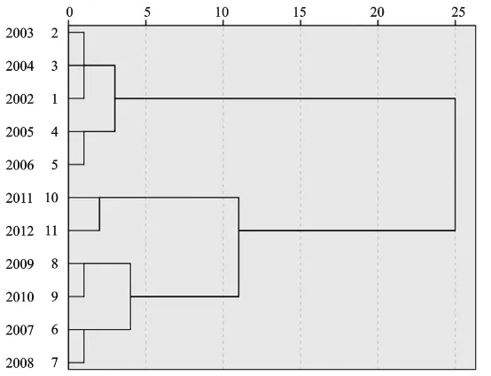
of 2002 as 100, and recalculated cpi from 2002 to 2012. Then dividing the original data by recalculated cpi, and multiplying it by 100, finally we obtained the per capita disposable income panel data and the per capita cash expenditure panel data eliminated the rising factor of price. Using SPSS 19.0, we carried out clustering analysis of the panel data respectively. The following is the comparison of the cluster tree.
From Figure 1, we can classify the per capita disposable income from 2007 to 2012 into the same cluster. From Figure 2, we can classify the per capita cash expenditure from 2007 to 2012 into the same cluster. There-fore, we can build panel data model on the per capita disposable income and the per capita cash expenditure of Chinese urban residents’ eight income levels from 2007 to 2012.
2Random disturbance term is divided into relevant case and irrelevant case.
3
Data is from China statistical yearbook (2003-2013).
4
255
Figure 1. Clustering tree of per capita disposable income panel data (2002-2012).
[image:5.595.150.534.93.445.2]Figure 2. Clustering tree of per capita cash expenditure panel data (2002-2012).
Table 1 and Table 2 are two original panel data from 2007 to 2012. Because China’s cpi is calculated based the previous year as the base period 100, not based a certain date as the base period, we needed to recount cpi
since 2007. The calculation results are shown in Table 3. We needed to eliminate the rising factor of the panel data in Table 1 and Table 2. Then it could be put into the model. Namely dividing the original data by recalcu-lated cpi in Table 3 respectively, and multiplying it by 100.
3.2. Build Model
Due to the structure of consumption and income from 2007 to 2012 belongs to the same type, so we can set the model parameters as unaffected by time. The form is:
, 1, ,8, 2007, , 2012. it i it i it
y =α +x β +u i= t= (6)
[image:5.595.177.454.321.533.2]256
Table 1. Per capita disposable income of Chinese urban residents (RMB).
Income levels 2007 2008 2009 2010 2011 2012
Poor households 3357.9 3734.4 4197.6 4739.2 5398.2 6520
Lowest income households 4210.1 4753.6 5253.2 5948.1 6876.1 8215.1
Lower income households 6504.6 7363.3 8162.1 9285.3 10,672 12488.6
Lower middle income households 8900.5 10195.6 11243.6 12702.1 14498.3 16761.4
Middle income households 12042.3 13984.2 15399.9 17224 19544.9 22419.1
Upper middle income households 16385.8 19254.1 21018.0 23188.9 26,420 29813.7
Higher income households 22233.6 26250.1 28386.5 31,044 35579.2 39605.2
[image:6.595.86.542.132.441.2]Highest income households 36784.5 43613.8 46826.1 51431.6 58841.9 63824.2
Table 2. Per capita cash expenditure of Chinese urban residents (RMB).
Income levels 2007 2008 2009 2010 2011 2012
Poor households 3447.7 3862.7 4256.8 4715.3 5575.6 6366.8
Lowest income households 4036.3 4532.9 4900.6 5471.8 6431.9 7301.4
Lower income households 5634.2 6195.3 6743.1 7360.2 8509.3 9610.4
Lower middle income households 7123.7 7993.7 8738.8 9649.2 10872.8 12280.8
Middle income households 9097.4 10344.7 11309.7 12609.4 14028.2 15719.9
Upper middle income households 11570.4 13316.6 14964.4 16140.4 18160.9 19830.2
Higher income households 15297.7 17888.2 19263.9 21000.4 23906.2 25796.9
Highest income households 23337.3 26982.1 29004.4 31761.6 35183.6 37661.7
Table 3.Recalculated cpi values based cpi of 2007 as 100.
Year 2007 2008 2009 2010 2011 2012
cpi 100 105.6 104.6 107.9 113.6 116.7
rising factor of price based cpi of 2007 as 100. In addition, due to the model studied each income group’s own data, so the parameters can be regarded as fixed parameters to estimate. Namely the model is the fixed effect model.
3.2.1. Model Identification
Using Eviews 7.0 to respectively calculate the sums of residual squares for variable coefficient model, variable intercept model and basic model under ordinary least square method (the calculation results is in Table 4), and putting N = 8, T = 6, K = 1 together into test statistics F2, F1, and comparing with the critical value under the significance level α =0.05, thus determining the model form.
The values of F F2, 1 are calculated as follows:
(
) (
)(
)
(
)
(
) (
) (
)
(
)
3 1
2
1
1 1 8294394 978731 8 1 1 1
17.08
1 978731 8 6 1 1
S S N K
F
S N T K
− − + − − × +
= = =
− − × − −
(
) (
)
(
)
(
) (
)
(
)
2 1
1 1
1 2882910 978731 8 1 1
8.89
1 978731 8 6 1 1
S S N K
F
S N T K
− − − − ×
= = =
− − × − −
Comparing with the critical value:
(
)(
) (
)
(
)
(
)
0.05 1 1 , 1 0.05 14, 32 0.05 15, 30 2.01 17.08
F N− K+ N T− −K =F ≈F = <
(
)
(
)
(
)
(
)
0.05 1 , 1 0.05 7, 32 0.05 7, 30 2.33 8.89
F N− K N T− −K =F ≈F = <
257
3.2.2. Parameter Estimation
Assuming that random disturbance items are irrelevant in different cross section individuals, then we can take each time series as sample, and use ordinary least squares method to estimate βi. The following are the para-meter estimation results.
From Table 5, we can conclude that the marginal consumption propensity is decreasing and the intercept item is increasing with the improvement of income level. From Table 6, we can learn that the goodness of fit of the model is as high as 99.9%. It indicates that the fitting effect of fixed effect variable coefficient model is very good. Statistics F also passed the test of significance. It indicates that the regression equation is significant as a whole, and the regression coefficients are significant. It shows that income has significant effect on consumption under each income level. The value of statistic DW is close to 2, so there is no first-order autocorrelation in the random error term uit5, which is consistent with the hypothesis, thus the process of modeling and the results are believable.
3.3. Results Analysis
By the parameter estimation results, the following conclusions can be drawn:
1) When income levels are different, there are obvious differences in marginal consumption propensity. And the marginal consumption propensity is decreasing with the improvement of income level. It shows that income disparity exactly is the decisive factor in influencing consumption, and the higher the income is, the weaker the marginal consumption desire is. That is consistent with the saying “diminishing marginal returns” in economics.
Table 4. Sums of squared residuals of the three models.
Model forms Variable coefficient model ( )S1 Variable intercept model ( )S2 Basic model ( )S3
[image:7.595.89.543.342.642.2]Sum of squared residuals 978,731 2,882,910 8,294,394
Table 5. The estimation results of the variable coefficient model.
Income levels Marginal consumption propensity ( )βi Intercept ( )αi
Poor households 0.916095 −1431.855
Lowest income households 0.80146 −1154.611
Lower income households 0.628855 −324.979
Lower middle income households 0.625534 −265.0764
Middle income households 0.619132 −166.872
Upper middle income households 0.606672 −71.132 95
Higher income households 0.59452 370.0824
Highest income households 0.505467 3044.444
Table 6. The statistical results of the variable coefficient model.
Cross-section fixed (dummy variables)
R-squared 0.999665 Mean dependent var 12181.09
Adjusted R-squared 0.999508 S.D. dependent var 7882.601
S.E. of regression 174.8867 Akaike info criterion 13.42735
Sum squared resid 978,731 Schwarz criterion 14.05109
Log likelihood −306.2565 Hannan-Quinn criter 13.66306
F-statistic 6363.363 Durbin-Watson stat 1.97787
Prob(F-statistic) 0.000000
5The value of statistic DW is between 0 and 4. Generally speaking, when the value is close to 0, there is a positive first-order autocorrelation
258
2) The intercept item is increasing with the improvement of income level. It shows that the absolute consump-tion level of urban residents is increasing by increased income.
3) In general, the marginal consumption propensity of different income levels is over 50%. It shows that no matter what the income levels of residents are, their consumption desire is very high. But different income levels may pursue different consumption direction.
4. Conclusion
Panel data model could analyze practical problems from the angles of time and the individual, so its application is becoming wider and wider. General theory about panel data has been relatively mature, and general linear panel data model was applied in this paper. According to the intercept item and marginal consumption propen-sity of variable coefficient panel data model, we can distinguish the spending habits in recent years between dif-ferent income levels, and then introduce difdif-ferent policies to stimulate consumption. But this paper didn’t subdi-vide consumption into different directions, such as: food, clothing, household goods, etc. If we join these aspects into the model, the results will be more beneficial for stimulating consumption. And general panel data model could finish the idea. Additionally, we still need to study nonclassical panel data models, such as: dynamic panel data model and nonlinear dynamic panel data model. Long and Zhang [14] studied theory and application of dynamic panel data model. But its parametric and nonparametric estimations still need to be studied further.
Acknowledgements
The authors would like to thank for the assistance provided by Hongfu Pan and Guoshuai Wang. They suggested us the journal and told us online submission. We finally finished the paper with their concern.
References
[1] Li, Z.N. and Pan, W.Q. (2010) Econometrics. 3rd Edition, Higher Education Press, Beijing.
[2] Yu, G. (2011) Research on the Parameter Estimation Problems of Panel Data Models. Ph.D. Thesis, Northeast Normal University, Changchun.
[3] Campbell, J.Y. and Mankiw, N.G. (1991) The Response of Consumption to Income: A Cross-Country Investigation.
European Economic Review, 35, 723-767. http://dx.doi.org/10.1016/0014-2921(91)90033-F
[4] Islam, M.N. (1995) Growth Empirics: A Panel Data Approach. Quarterly Journal of Economics, 110, 1127-1170.
http://dx.doi.org/10.2307/2946651
[5] Hsiao, C. (2003) Analysis of Panel Data. 2nd Edition, Peking University Press, Beijing.
http://dx.doi.org/10.1017/CBO9780511754203
[6] Baltagi, B.H. (2005) Econometric Analysis of Panel Data. 3rd Edition, John Wiley &Sons Inc., New York.
[7] Chen, H.Y. (2006) Analysis and Application of Panel Data. M.S. Thesis, Tianjin University, Tianjin.
[8] Chen, H.Y. (2010) Research on the Testing Methods in Panel Data Models. Ph.D. Thesis, Tianjin University, Tianjin.
[9] Bai, Z.L. (2010) Setting, Statistical Test and New Progress of Panel Data Model. Statistics and Information Forum, 25, 3-12.
[10] Zhu, W. and Li, Y.S. (2006) Panel Data Analysis of China Urban Residents’ Consumption Structure. Application of Statistics and Management, 25, 645-648.
[11] Chen, H.Y., Yang, B.C. and Li, S.C. (2009) Analysis of Panel Data of Consumption Structure of Urban Residents in China .Statistics and Decision, 24, 112-114.
[12] Wang, L. (2012) Application of Panel Data Analysis Method in the Relationship between Income and Consumption of Our Country. M.S. Thesis, Lanzhou Jiaotong University, Lanzhou.
[13] Zhu, J.P. and Chen, M.K. (2007) The Cluster Analysis of Panel Data and Its Application. Statistical Research, 24, 11- 14.