Bounded Rationality and Socially Optimal Limits on Choice in A Self Selection Model

Munich Personal RePEc Archive

Bounded Rationality and Socially

Optimal Limits on Choice in A

Self-Selection Model.

Sheshinski, Eytan

The Hebrew University of Jerusalem

January 2000

ילשוריב תירבעה הטיסרבינואה

THE HEBREW UNIVERSITY OF JERUSALEM

BOUNDED RATIONALITY AND SOCIALLY

OPTIMAL LIMITS ON CHOICE IN

A SELF-SELECTION MODEL

by

EYTAN SHESHINSKI

Discussion Paper # 330

July 2003

ויצרה רקחל זכרמ

תוילנ

CENTER FOR THE STUDY

OF RATIONALITY

Bounded Rationality and Socially

Optimal Limits on Choice in

A Self-Selection Model

Eytan Sheshinski*

January 2000

Revised: November 2002

Abstract

When individuals choose from whatever alternatives available to them the one that maximizes their utility then it is always desirable that the government provide them with as many alternatives as pos-sible. Individuals, however, do not always choose what is best for them and their mistakes may be exacerbated by the availability of op-tions. We analyze self-selection models, when individuals know more about themselves than it is possible for governments to know, and show that it may be socially optimal to limit and sometimes to elimi-nate individual choice. As an example, we apply Luce’s (1959) model of random choice to a work-retirement decision model and show that the optimal provision of choice is positively related to the degree of heterogeneity in the population and that even with very small degrees of non-rationality it may be optimal not to provide individuals any choice.

JEL Classification: D11, D63, D81, H1.

Key Words: Logit, self-selection, moral-hazard, retirement. _____________________

1

Introduction

Providing choice to individuals is beneficial because it can satisfy

peo-ple’s varied tastes. Often, however, expanded choices lead to decision errors. Psychological studies of decision-making suggest that these errors and other

costs associated with the choice process1 _{can be significant and sometime}

outweigh the benefits conferred by a larger set of alternatives. This happens

particularly in areas where decision makers lack expertise and their evaluation requires complex calculations. Old-age pension programs is a relevant exam-ple. Savings for consumption during retirement involves many interrelated uncertainties. Long-ranged discounting and annuitization depend critically on personally uncertain attributes such as health, mortality rates and future

earnings, as well as macro variables such as interest rates. It is difficult to

evaluate these uncertainties early in life as they unfold long after decisions are made.

Insurance policies offered by government cannot be based on individual

characteristics because individuals do not willingly reveal their full character-istics. The government can reasonably know the distribution of characteristics

within the population and will devise its policy to best fit this distribution,

taking into account individuals’ self-selection among alternative programs available to all. This ‘Second-Best’ social optimum typically provides for a range of choice to individuals. It is interesting to inquire whether relaxing the assumption of fully rational choice by individuals due to reasons such as those discussed above, removes or limits the presumption that provision of

choice is socially desirable. This question was first raised by Mirrlees (1987),

who provided some insightful examples of non-rationality leading to socially optimal policy which leaves no choice to individuals.

1_{Lowenstein (2000) identifies three types of costs associated with the evaluation of}

alternatives: the opportunity costs of the time it takes; the tendency to make errors

Luce (1959) proposed a model of ‘bounded-rationality’ in which individ-uals attempt to maximize utility but make errors in the decision process. These errors lead to random deviations of the chosen alternative from the

best, reflecting utility maximization imperfectly. This is the well-knownLogit

model. One merit of the model is that it allows a convenient measure of the degree of non-rationality, which is the focus of our analysis.

In this paper we apply Luce’s model to a situation in which

individ-uals have to choose between work and no-work (retirement). When offered

consumption levels for workers and non-workers, individuals with varying de-gree of labor disutility probabilistically self-select themselves between work and non-work. The government’s objective is to choose consumption levels that maximize a utilitarian social welfare function subject to a resource con-straint. The optimal policy depends on individuals’ degree of non-rationality.

When fully rational, it is always optimal to offer them choice. However, we

demonstrate that with some degree of non-rationality, the elimination of the retirement (or work) option may be socially optimal. Calculations based on standard functional forms demonstrate that this elimination of choice be-comes optimal at surprisingly low levels of non-rationality.

The government is assumed to pursue a socially optimal policy. With less than rational behavior by the government, it may be desirable to design a constitution which limits the choices available to such government. This, in turn, may further restrict the provision of choice to individuals. We plan to study this question in a subsequent paper.

In the context of the current debate about reforming social security with

provision of more choice to individuals, our calculations suggest that benefi

2

The Luce Model

Consider an individual who has to choose one among a set of mutually

exclusive alternatives. Neoclassical economic theory assumes that the indi-vidual has a utility function that allows him or her to rank these alternatives,

choosing the highest ranked. Psychologists (e.g. Luce (1959), Tversky (1969)

and (1972)) criticized this deterministic approach, arguing that the outcome

should be viewed as a probabilistic process. Their approach is to view utility

as deterministic but the choice process to be probabilistic. The individual

does not necessarily choose the alternative that yields the highest utility and

instead has a probability of choosing each of the various possible alternatives.

A model of ‘bounded rationality’ along these lines has been proposed by Luce (1959). Luce shows that when choice probabilities satisfy a certain

axiom (the ‘choice axiom’), a scale, termed ‘utility’, can be defined over

alternatives such that the choice probabilities can be derived from the scales

(‘utilities’) of the alternatives.

Consider a set S of a finite number, n, of discrete alternatives, ai, i =

1, 2..., n. Luce’s (Multinomial) Logit Model postulates that the probability

that an individual chooses some alternativeai ∈S, pS(ai), is given by

pi =pS(ai) =

equi

n

P

j=1

equj

, i= 1, 2..., n (1)

whereui =u(ai)for some real-valued utility functionu, andqis a positive

constant representing the ’precision’ of choice. Whenq = 0, all alternatives

2_{For a comprehensive discussion of discrete choice theory see Anderson, de-Palma and}

have an equal probability to be chosen: pi = 1_n for all i = 1,2..., n. As q

increases to +_∞, pi increases monotonically, approaching 1, when ui is the

largest among all uj, j = 1, 2, ..., n, and decreases monotonically,

approach-ing 0, otherwise. Thus, it is natural to call the parameter q the ’degree of

rationality’ (with q=∞called ’perfect rationality’).3

3_{Debreu (1990) has pointed out a weakness in Luce’s model. The introduction of}

a new alternative “more than proportionately reduces the choice probabilities of existing alternatives that are similar, while causing less than proportionate reductions in the choice probabilities of dissimilar alternatives” (Anderson,et-al (1992)). This is the well-known “blue bus/red bus” paradox. This objection, can be pertinent in imperfectly competitive market circumstances, when firms may take advantage of this implication. In the social welfare context, on the other hand, the government may take advantage of this property in providing weight to socially desirable ’default’ alternatives. Generally, Luce’s model has considerable merit as it incorporates a tendency to utility maximization and the parameter

3

Social Welfare Analysis

Suppose that the population consists of heterogeneous individuals, each

characterized by a parameter θ. Individual θ’s utility of alternative i is

ui(θ) = u(ai, θ), with the corresponding choice probabilities pi(θ) given by

(1), i = 1, 2, ..., n. We postulate (Mirrlees (1987)) that individuals’ welfare

is represented by expected utility, V(θ),

V(θ) =

n

X

i=1

pi(θ)ui(θ) (2)

We assume that all individuals have the sameq4 _{and that social welfare,}

W, is utilitarian:

W(q) =

Z

V(q)dF(θ) =

Z "_Xn i=1

equi_u

iÁ n

X

j=1

equj

#

dF(θ) (3)

where F(θ) is the distribution function of θ in the population. The

gov-ernment’s objective is to choose policies that maximizeW subject to relevant

resource constraints and taking into account individual reactions to alterna-tive policies. We begin by assuming that individuals are passive, i.e. they only choose alternatives probabilistically as described above and there are no

resource constraints5_.

4_{It is interesting to analyze the case of different group levels ofq. Individual ’awareness’}

of their own and of others’ levels of q and the corresponding market interactions and strategies become then crucial issues.

5_{It is easy to incorporate resource constraints when they are at the individual level.}

Thus, suppose that when choosing alternativei, individualθ’s utility isui(xi, y,θ), where

xi is an attribute of alternativei to be chosen by the individual andy is the quantity of

a numeraire good. With given income R(θ) and a private cost ci(xi,θ)of alternative i,

y=R(θ)₋ci(xi,θ) (≥0). The utilityui(θ)in the text can be interpreted as theoptimized

utility (w.r.t. xi) which incorporates the resource constraint. See below on the case when

LetV(θ)be the utility of individualθ when choosing the best alternative:

V(θ) =argmax[u1(θ), u2(θ), ..., un(θ)] (4)

The corresponding level of social welfare when each individual chooses

his/her best alternative, W, is

W =

Z

V(θ)dF(θ) (5)

Denote by Wi the level of social welfare when all individuals choose

al-ternative i:

Wi =

Z

ui(θ)dF(θ) (6)

We now state:

Proposition 1. (I)If all alternatives do not yield the same utility for all

individuals, then W(q) strictly increases in q; (II) W(_∞) = lim

q→∞W(q) = W

and (III)W(0) = lim

q→0W(q) = 1

n

n

P

i=1

Wi.

Proof. Using the definitions (1), (2) and (3), it can be shown that

dW(q)

dq =

Z "_Xn i=1

(ui(θ)−V(θ))2pi(θ)

#

dF(θ), (7)

which, under the assumption, proves (I). Statements (II) and (III) also

Under ’perfect-rationality’, q = _∞, each individual makes the ’right choice’, and hence there is no reason, from a social welfare point of view, to limit the choice set. By continuity, this conclusion applies to large levels

ofq. When individuals make small errors, the full set of alternatives can best

accommodate the diversity of individual preferences represented byθ. At the

other extreme, when all alternatives have equal probabilities to be chosen by

all individuals, q = 0, a large set of alternatives exacerbates (’spreads’) the

errors that individuals make to an extent that clearly outweighs the

bene-fits of diversity. It is then socially optimal to drastically reduce the set of

alternatives to a singleton, i.e. not to provide individuals any choice. This single socially preferred alternative depends, of course, on the distribution of population characteristics, accommodating as large as possible a mass con-centration of individuals. The proof of this statement is straightforwards.

Let

Wm ⊆arg max(W1, W2, ..., Wn) (8)

In case of ties, the following applies to any element in the set (8). We now have:

Proposition 2. If Wi, i= 1, 2, ..., n are not all equal, then when q = 0

social welfare is maximized by offering only alternative m.

Proof. Follows directly from the fact thatW(0) = 1

n

n

P

i=1

Wi and from (8)

¥.

Since W(q) is continuous in q, the implication of Proposition 2 is that

there exists a positive level ofq, sayq0, such that for allq ≤q0, restricting the

choice set confronting individuals to alternative malone is socially desirable.

As q increases above q0, it is desirable to expand the set of alternatives,

this ’expansion process’ is gradual, i.e. whether it is optimal to include one

or more alternatives simultaneously as q increases from q06.

It can be shown that all these cases are possible. Here we shall focus

only on q0, characterizing the extent of errors that warrant the elimination

of individual choice.

6_{Let T be a subset of {1,2, , n}, standing for the indices of the alternatives offered}

to individuals. Consider the addition of alternative s, not included in T. Denote by

T0 _{=sU T, and letW}T

and WT0 _{be the corresponding levels of social welfare when the}

alternatives inT(T0_{)are offered to individuals. It can be shown that} WT0

−WT

=R pT0

s (θ)(us(θ)−V T

(θ)dF(θ)), wherepT0

s (θ)is the probability that

indi-vidualθchooses alternativeswhen confronting the setT0 _andVT

(θ)is expected utility of individual θwhen confronting the setT. A necessary and sufficient condition forsto be included in the socially optimal set for someqis that, for some subsetT,us(θ)−V

T

(θ)>0

in an interval ofθ with a positive density. Sufficiency follows from the fact that asq in-creases,pT0

s (θ)approaches zero for thoseθfor whichus(θ)−V T

(θ)<0and approaches 1 on the complementary set ofθ.

Starting with a single alternative atq=q0, one can formulate an algorithm for inclusion

4

Self-Selection and Aggregate Constraints

The model outlined above has the property that, under perfect rationality

(q = ∞), the economy attains the First-Best allocation of resources when

individuals are offered the complete set of alternatives. At the other

ex-treme, we concluded that when individual choice probabilities are uniformly

distributed (q = 0), it is socially optimal to eliminate individual choice.

Both conclusions have to be modified when the model incorporates private

information not available to the government whose policies affect individual

choice. The argument, however, that it is socially advantageous to reduce the choice set confronting individuals as they make increasing errors is still valid.

Suppose that the individual characteristic θ is private information, the

government having only information on the distribution F(θ). Government

policies affecting individual utilities and choice probabilities cannot therefore

depend on θ. It is well-known that in these circumstances, even when

indi-viduals are perfectly rational, optimal policies lead to a Second-Best

(’Self-Selection’) equilibrium. When individuals are boundedly rational, the

so-cially optimal policies have to take into account their effect on the choice

probabilities. This leads, in particular, to a modification of the conclusion

that when probabilities are uniformly distributed (q = 0) it is always

opti-mal to eliminate individual choice. This stark result may still be optiopti-mal,

but other optimal configurations are possible. The reason is that, under an

aggregate resource constraint, the government’s optimal policies are different

when a single alternative is offered than when a number of alternatives are

permitted.

Letui =ui(xi, θ),i= 1, 2, ..., n, be individualθ’s utility of alternativei,

wherexi is some government policy (independent ofθ). Choice probabilities,

pi = pi(xi, θ), and expected utility

n

P

i=1

pi(xi, θ)ui(xi, θ) all depend on xi.

welfare subject to a resource constraint

Z "_Xn i=1

pi(xi, θ)ci(xi)

#

dF(θ) =R (9)

where ci(xi) is the cost of xi in terms of the given level of the aggregate

resource, R. Denote the policies that maximize W subject to the resource

constraint (9) by x_bi(q), i = 1, 2, ..., n, and the corresponding level of social

welfare by Wc(q):

c

W(q) =

Z "_Xn i=1

pi(xbi(q),θ)ui(bxi(q), θ)

#

(10)

A full-information policy would make xi depend on θ and hence Wc(∞)

is a Second-Best equilibrium.

Whenq= 0,

c

W(0) = 1

n

n

X

i=1

Wi(xbi(0)) (11)

where Wi(xbi(0)) =

R

ui(bxi(0), θ)dF(θ), and xbi(0) is the limit of bxi(q) as

q →0.

Let exm be the feasible policy when only alternative m is permitted. By

(9), it is the solution to cm(xem) = R. The corresponding social welfare

is Wfm =

R

um(xem)dF(θ). It is seen that even if Wm(bx(0)) = arg max

[W1(bx1(0)), W2(xb2(0)), ..., Wn(bxn(0))], it does not follow necessarily thatWfm >

c

W(0)7_{. Eliminating choice atq≤q}

0 is now only one of a number of possible

outcomes.

Rather than develop sufficient conditions for the single outcome, we turn

to a detailed example that incorporates the above considerations.

5

A Work-Retirement Model

Individuals can choose whether to work or retire. We take work to be a

0₋1variable and do not model varying hours or work intensity. All workers

are assumed to have the same (non-negative, increasing and concave) utility

of consumption, u(c), while all non-workers have (non-negative, increasing

and concave) utility of consumption, v(c)8_{. Disutility of work, denoted θ,}

is assumed to be additively separable from consumption, so the utility of a

worker with labor disutility level θ is written u(ca)−θ. The distribution of

disutilities plays a central role in determining the willingness to work.

We consider two different consumption levels: cafor active workers andcb

for non-workers (”retirement benefits”). We assume that θ is distributed in

the population with distribution F(θ) (and density f(θ)). For convenience,

we assume that f(θ) is continuous and positive for all non-negative values

of θ. Having individuals with a very large labor disutility implies, of course,

that some will choose not to work.

Each worker is assumed to produce one unit of output. Thus, if all

in-dividuals with labor disutility less than some value, θ0, work, the economy’s

resource constraint is θ0

Z

0

(ca−1)dF(θ) + ∞

Z

θ0

cbdF(θ) =R, (12)

where R is the level of outside resources available to the economy. It is

as-sumed, of course, that R >₋1to enable positive consumption.

5.1

First-Best (Labor Disutility Observable)

To set the stage for the optimal policy when labor disutility is not

ob-servable, it may be useful to analyze first the full optimum where disutility

is observable.

The government’s objective is to maximize a utilitarian social welfare

function, W,

W =

θ0

Z

0

(u(ca)−θ)dF(θ) + ∞

Z

θ0

v(cb)dF(θ), (13)

subject to the resource constraint (12). Optimal consumption, c∗

a and c∗b, is

allocated so as to equate the marginal utilities of consumption of workers and non-workers

u0_(c∗

a) =v0(c∗b) (14)

All individuals with disutility below a cutoff, denoted θ∗, should work. The

cutoff is determined by comparing the utility gain from extra work,u(c∗

a)−

θ∗₋u(c∗

b)with the value of extra net consumption as a consequence of work,

which is the sum of the marginal product and the change in consumption which results from the change in status:

u(c∗_a)₋θ∗₋v(c∗_b) =u0_(c∗

a)(1−c∗a+c∗b) (15)

Whether the solution is interior, θ∗ > 0, depends on the wealth of the

economy, i.e. the size ofR. If no one works, optimal consumption isc∗b =R.

This allocation is not optimal if those with no labor disutility9_{, when put}

to work for additional consumption equal to their marginal product, enjoy a higher utility

u(R+ 1)> v(R) (16)

9_{This assumes that f(θ)>0at θ = 0. Otherwise, a condition similar to (16) below}

has to be assumed with respect to those with the least (positive) labor disutility for which

We assume that (16), which Diamond and Sheshinski (1995) call the

‘poverty condition’, is satisfied. This condition ensures that there is some

work at the optimal allocation10_{. It can also be seen that it is always optimal}

for some individuals not to work11_.

5.2

Labor Disutility Unobserved

Assume now that individuals choose whether they prefer working to

receiving retirement benefits, or vice-versa. Those with disutilities of labor

below a threshold value which equates utilities of workers and non-workers

will choose to work. The threshold value,bθ, satisfies

b

θ =Max[0, u(ca)−v(cb)]. (17)

The government’s problem is now restated as selection ofcaandcb so as to

maximize (13) subject to (12), withθ0 not an independent choice parameter

but replaced bybθ, (17), which is a function of ca andcb.

Using the Lagrange multiplier λ and assuming an interior solution, we

can state the first-order conditions as the resource constraint, (12), and the

following two equations:

(u0_(c

a)−λ) bθ

R

0

dF(θ) =λ(ca−1−cb)f(bθ)_dcdbθ

a

=λ(ca−1−cb)f(bθ)u0(ca)

(18)

(v0_(c

b)−λ) ∞

R

b

θ

dF(θ) =λ(ca−1−cb)f(bθ)_dcdbθ

b

=−λ(ca−1−cb)f(bθ)v0(cb)

(19)

10_{By (12), when θ}∗_{= 0,c}∗

b =R. Setting c∗a =R+ 1, condition (16) implies that the

L.H.S. of (15) is larger than the R.H.S.(= 0).

11_{If there are no non-workers thenc}∗

b = 0 andc∗a=R+ 1. It follows from (15) that the

where we have used (17) to obtain the derivatives of bθ. The L.H.S. of (18) and (19) are the net social values of giving consumption to workers and non-workers, respectively, rather than holding the resources. The R.H.S. are the social values of the resource savings from the induced changes in labor supply

as a result of changes in ca andcb, respectively. The private return to work

is ca−cb and hence, since the marginal product is one,1−ca+cb >0 is an

implicit tax on work.

Denote by (_bca,bcb) optimal consumption which solves (18) and (19) and

denote by bλ the corresponding optimal Lagrangean. Dividing (18) by u0_(bc

a)

and (19) by v0_(bc

b)and adding these equations, we get

b

λ−1 = (u0_(bc

a))−1 bθ

Z

0

dF(θ) + (v0_(bc

b))−1 ∞

Z

bθ

dF(θ) (20)

That is, the inverse of the Lagrangian is a weighted average of the inverse of

the marginal utilities at the optimum, u0_(bc

a) andv0(bcb).

We shall now impose a condition that will imply that, at the optimum, the marginal utility of consumption of non-workers exceeds that of workers.

This is the Diamond-Mirrlees (1978) moral-hazard condition, that equating

utilities between non-workers and workers who dislike work the least leaves marginal utility higher for non-workers:

u(x) =v(y) implies u0_{(x)< v}0_{(y). (21)}

Since bθ >0, (17) implies that u(bca) > v(bcb). Hence,by (21), u0(bca) < v0(bcb).

By (20) then, u0_(bc

a)<λ < v0(bcb), and it follows from (18)-(19) that 1−bca+

b

6

Logit Model of Randomness in Individual

Decisions

Instead of the previous deterministic model of individual choice,

sup-pose now that an individual with labor disutility θ chooses to work with

probability pa, where

pa=pa(ca, cb, q,θ) =

eq(u(ca)−θ)

eq(u(ca)−θ)+eqv(cb), (22)

This is a special case of the logit model presented in Sections 2 and 3.

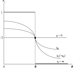
It is seen that as q, the degree of accuracy (‘rationality’), increases from 0

to +_∞, pa increases (decreases) from pa = 1₂ for all θ to pa = 1(= 0) for

θ <(>)bθ =u(ca)−v(cb)>012. Figure 1 depictspa as a function ofθ.

The sum of the probabilities of all individuals who should work, that is

those with θ <bθ =u(ca)−v(cb), relative to this sum under full rationality

(=bθ), can be viewed as an indicator for the effects of ‘bounded-rationality’.

Appendix A provides some calculations for representative values of ca, cb

and alternative values of q. For the case u(c) =v(c) = lnc, this proportion

depends on the ratio cb/ca. With cb/ca =.5, it increases from .5 to .97 as q

increases from 0 to 30. With cb/ca=.7 it reaches .94 and withcb/ca =.9it

reaches only .79, at q= 30. Thus, a highercb/ca has a significantly negative

effect on this proportion.

With choice of work and retirement governed by the probabilities pa,

social welfare is expressed as the sum of expected utilities:

W =

∞

Z

0

[(u(ca)−θ)pa+v(cb)(1−pa)]dF(θ). (23)

12_Whenu(c

Accordingly, the resource constraint is given by

∞

Z

0

[(ca−1)pa+cb(1−pa)]dF(θ) =R. (24)

Maximization of (23) with respect to ca and cb subject to (24), taking

into account the dependence ofpaon these variables, (22), yields, in addition

to (24), first-order conditions:

(u0_(c

a)−λ) ∞

R

0

padF(θ)

=R∞ 0

[λ(ca−1−cb)−(u(ca)−θ−v(cb))]∂_∂p_ca

bdF(θ)

=R∞ 0

[λ(ca−1−cb)−(u(ca)−θ−v(cb))]

pa(1−pa)qu0(ca)dF(θ)

(v0_(c

b)−λ) ∞

R

0

(1−pa)dF(θ)

=R∞ 0

[λ(ca−1−cb)−(u(ca)−θ−v(cb))]∂_∂p_ca

bdF(θ)

=−R∞

0

[λ(ca−1−cb)−(u(ca)−θ−v(cb))]

(25)

pa(1−pa)qv0(cb)dF(θ), (26)

where we used that ∂pa

∂ca =qpa(1−pa)u

0_(c

a)and ∂_∂p_ca_b =qpa(1−pa)v0(cb).

The interpretation of these conditions is basically unchanged: the L.H.S. of (25) and (26) is the expected net value of additional consumption to work-ers and non-workwork-ers, respectively. The R.H.S. is expected next resource cost

of this additional consumption, which now includes the effect on all

negative) of a change in the probability of work as a result of the change in consumption.

Denote the optimal consumption levels which solve (24), (25) and (26)

by (bca(q),cbb(q)). These levels imply, in turn, an optimal probability pba =

b

pa(q,θ) =pba(cba,bcb, q,θ) for an individual with labor disutilityθ to choose to

work. The corresponding optimal level of social welfare, denoted cW(q), is

given by (23): Wc(q) =R∞

0

[(u(_bca)−θ)bpa+v(bcb)(1−pba)]dF(θ).

We shall be interested in the dependence of these optimal values on the

degree of rationality, q.

Asq goes to +_∞, p_ba approaches 1 or 0 depending on whetherθ is below

or above bθ, (17), while qp_ba(1−bpa)dF(θ) approaches f(bθ)dθ for θ = bθ and

0 elsewhere. Thus, (25)-(26) are a generalization of (18)-(19), converging to

the latter as q goes to +∞.

Dividing (25) and (26) byu0_(bc

a)andv0(bcb), respectively, and adding these

equations we get:

b

λ−1 _{= (u}0_(bc

a))−1 ∞

Z

0

b

padF(θ) + (v0(bcb))−1 ∞

Z

0

(1₋p_ba)dF(θ) (27)

7

Dependence of the Optimum on the Degree

of Rationality

When individuals have a choice between work and retirement, the

op-timal level of social welfare, cW(q), increases with the degree of rationality,

dcW

dq >0, provided we assume that, for all q, there is an implicit optimal tax

on work: 1_−bca+bcb >0(Appendix B). At one extreme, when individual

de-cisions are fully rational and deterministic,q = +_∞, it is always optimal for

some individuals with low labor disutility to work (the ‘poverty condition’, (16)) and for some with large labor disutility to retire (we have assumed

that f(θ)>0for all positive θ). At the other end, whenq = 0, individuals’

choice between work and retirement is independent of the levels of ca andcb,

being pa = 1₂ for all θ. That is, half of all individuals choose not to work,

including those with very low labor disutility. It seems possible, therefore,

that with relatively lowq, the elimination of the retirement option altogether

may dominate all feasible positive combinations ofca andcb. Similarly, since

half of all individuals choose to work, including those with very high labor disutility, it seems possible that the elimination of the work option may also

dominate all feasible positive combinations of ca and cb.

We want to demonstrate that these are valid possibilities:

Proposition 3. When q = 0 the optimal allocation has one of the

fol-lowing forms: (a) consumption levels of workers and of non-workers equate their marginal utilities, u0_(bc

a) = v0(bcb), and bca +bcb = 2R + 1; or (b) the

retirement option is eliminated, setting _bca=R+ 1; or (c) the work option is

eliminated, setting _bcb =R.

Inspection of (23) and (24) shows that in the presence of work and

retire-ment options, when q = 0 and pa = 1₂ for all ca, cb and θ, W is maximized

u0_(bc

a(0)) =v0(bcb(0)) wherebca(0) +bcb(0) = 2R+ 1 (28)

The corresponding welfare level, cW(0), is:

c

W(0) = 1

2[u(bca(0) +v(bcb(0))]− 1

2E(θ) (29)

where E(θ) =R∞

0

θdF(θ)is expected (‘average’) labor disutility.

Without a retirement option, bca =R+ 1 and the corresponding level of

welfare, denoted Wa, is

Wa =u(R+ 1)−E(θ) (30)

Without a work option, _bcb = R and the corresponding level of welfare,

denoted Wb, is

Wb =v(R) (31)

We want to show that each of (29), (30) or (31) is a possible optimum.

For this purpose, it suffices to examine a special case. Thus, assume that

u(c) =v(c). Then, from (28),_bca=bcb =R+₂1 andWc(0) =u(R+₂1)−1₂E(θ).

Elimination of the retirement option is optimal iffWa >Wc(0). By (29) and

(30), the following condition has to hold:

u(R+ 1)₋E(θ)> u(R+1 2)−

1

2E(θ) (32)

or

u(R+ 1)₋u(R+1 2)>

1

By concavity,u(R+1)₋u(R+1₂)> 1₂u0_{(R+1), hence asu}ffi_{cient condition}

for (33) is

u0_{(R+ 1)> E(θ). (34)}

By (30) and (31), Wa > Wb is equivalent to u(R+ 1)−u(R) > E(θ).

Hence, condition (32) is also sufficient for no-retirement to dominate the

no-work program.

Similarly, from (29) and (31),Wb >cW(0), iff

u(R)> u(R+1 2)−

1

2E(θ) (35)

or

u(R+1

2)−u(R)< 1

2E(θ) (36)

Since u(R+1

2)−u(R)< 1

2u0(R), a sufficient condition for (36) is

u0_{(R)< E(θ) (37)}

Again, (37) implies that Wb > Wa, that is, eliminating the work option

is optimal. Obviously, (34) and (37) are mutually exclusive: either a no-retirement program or a no-work program are optimal.

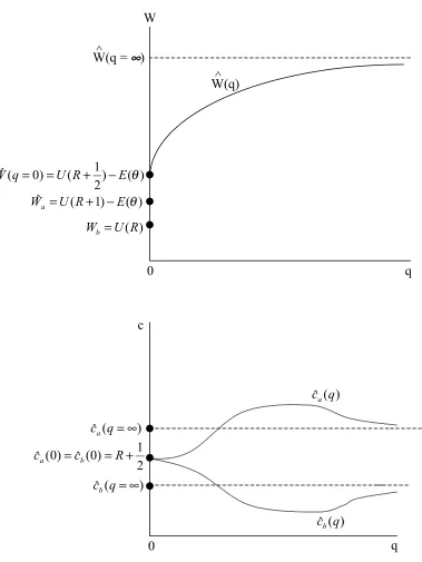
Calculations presented in the next section indicate the following

solu-tion pattern. As the degree of rasolu-tionality, q, decreases, so does the optimal

level of welfare,cW(q). The gap between optimal consumption of workers and

non-workers first increases in order to mitigate the rise in the probability of

errors due to lower rationality. However, at still lower levels of q, the gap

between workers’ marginal utility of consumption and that of non-workers becomes more important than the maintenance of low probabilities of error and consequently the consumption gap starts to decrease, eventually

disap-pearing (for u(c) =v(c)) when inevitable errors are unaffected by policy (at

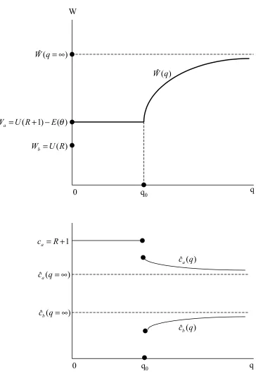
q = 0). Figure 2 presents this pattern which assumes thatcW(0)> Wa > Wb:

for all values of q. It is possible, however, as argued above, that

elimina-tion of the retirement opelimina-tion is dominant for small or moderate values of q

(Wa>cW(0)). This is depicted in Figure 3. Alternatively, it is possible that

elimination of the work option becomes dominant for small or moderate q.

8

Logarithmic Two-Class Example

Consider the case where there are only two types in the economy,θ1 and

θ2(θ1 < θ2), with population weights f1 and f2 = 1−f1. Let workers and

non-workers have the same logarithmic utility function: u(c) = v(c) = lnc.

Hence, workers and non-workers have equal consumption in the First-Best allocation. Accordingly, optimal social welfare when type one works and type

two retires, W∗

1 is

W∗ = ln(R+f1)−θ1f1. (38)

Social welfare when both types work,Wa, is

Wa= ln(R+ 1)−θ1f1−θ2f2 (39)

We shall assume that (38) is better than (39), which implies that

θ2 > 1

f2 ln

µ

R+ 1

R+f1

¶

(40)

Social welfare when nobody works, Wb, is

Wb = lnR (41)

We assumed that no work is inferior to type one working,W∗ > Wb (the

‘poverty condition’, (16)) which holds iff

θ1 < 1

f2 ln

µ

R+f1

R

¶

(which is trivially satisfied when θ1 = 013).

Under self-selection, the incentive compatibility condition for type one is

ln(ca)−θ1 ≥ lncb. Since the marginal utility of non-workers is higher than

that of workers, this condition holds with equality:

lnca−θ1 = lncb or ca =cbeθ1. (43)

Solving from the resource constraint

(ca−1)f1+cbf2 =R, (44)

we have

b

cb =

R+f1

eθ1f 1+f2

,bca=

eθ1(R+f 1)

eθ1f 1 +f2

(45)

With this allocation, social welfare,Wc(q=∞), is

c

W(∞) = ln

µ

R+f1

eθ1f 1+f2

¶

(46)

Comparing (46) and (49), the condition that at the self-selection optimum type two does not work is

θ2 > 1

f2

·

ln

µ

R+ 1

R+f1

¡

eθ1

f1+f2

¢¶

−θ1f1

¸

(47)

Conditions (40) and (47) are the same when θ1 = 0, otherwise (46) is a

somewhat more stringent condition than (40).

In the Logit model of Section 6, whenq = 0, half the population works

independent of the levels of consumption offered to workers and non-workers.

Hence, it is optimal to offer both equal consumption: bca(0) =bcb(0) =R+1₂.

As half the population works, social welfare,Wc(0), is accordingly

c

W(0) = ln(R+1 2)−

1

2(θ1f1+θ2f2) (48)

Without a retirement option, social welfare is given by (39). This level

exceeds (48) iff

θ2 < 1

f2

·

2 ln

µ

R+ 1

R+1₂

¶

−θ1f1

¸

(49)

For (46) and (49) to be mutually satisfied it is required that

(R+ 1)(R+f1)>(R+ 1 2)

2_(eθ1

f1 +f2) (50)

For example, withθ1 = 0, condition (48) is(R+1)f1 > 1₄. This can clearly

be satisfied. Thus, it is possible that a retirement alternative is desirable

when individuals select their best alternative with certainty, but it is socially optimal to eliminate this alternative when individuals are less than perfectly rational.

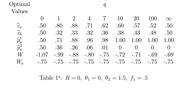
Since cW(q) increases in q14_{, whenever W}

a >cW(0) there exists a ‘cutoff’

q such that cW(q)is larger (smaller) than Wa forq larger (smaller) than this

value. It is interesting to examine at what level of q and the corresponding

optimal solutions this cutoffoccurs.

Optimal q

Values

0 1 2 4 7 10 20 100 _∞

bca .50 .80 .88 .71 .62 .60 .57 .52 .50

bcb .50 .32 .33 .32 .36 .38 .43 .48 .50

b

p1_a .50 .71 .88 .96 .98 1.00 1.00 1.00 1.00

b

p2a .50 .36 .26 .06 .01 0 0 0 0

W -1.07 -.99 -.88 -.80 -.75 -.72 -.71 -.69 -.69

Wa -.75 -.75 -.75 -.75 -.75 -.75 -.75 -.75 -.75

Table 1a_{: R= 0, θ}

1 = 0, θ2 = 1.5, f1 =.5

Optimal q Values

0 1 2 4 6 10 20 100 ∞

bca .5 .97 1.00 1.00 .95 .87 .80 .71 .67

bcb .5 .37 .43 .47 .50 .55 .60 .65 .67

b

p1_a .5 .72 .84 .95 .98 1.00 1.00 1.00 1.00

b

p2a .5 .37 .21 .05 .01 0 0 0 0

b

W -.94 -.80 -.65 -.52 -.50 -.44 -.42 -.41 -.41

Wa -.50 -.50 -.50 -.50 -.50 -.50 -.50 -.50 -.50

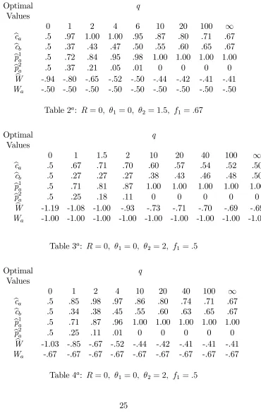
Table 2a_{: R = 0, θ}

1 = 0, θ2 = 1.5, f1 =.67

Optimal q

Values

0 1 1.5 2 10 20 40 100 ∞

bca .5 .67 .71 .70 .60 .57 .54 .52 .50

bcb .5 .27 .27 .27 .38 .43 .46 .48 .50

b

p1a .5 .71 .81 .87 1.00 1.00 1.00 1.00 1.00

b

p2_a .5 .25 .18 .11 0 0 0 0 0

b

W -1.19 -1.08 -1.00 -.93 -.73 -.71 -.70 -.69 -.69

Wa -1.00 -1.00 -1.00 -1.00 -1.00 -1.00 -1.00 -1.00 -1.00

Table 3a_{: R = 0, θ}

1 = 0, θ2 = 2, f1 =.5

Optimal q

Values

0 1 2 4 10 20 40 100 ∞

bca .5 .85 .98 .97 .86 .80 .74 .71 .67

bcb .5 .34 .38 .45 .55 .60 .63 .65 .67

b

p1_a .5 .71 .87 .96 1.00 1.00 1.00 1.00 1.00

b

p2a .5 .25 .11 .01 0 0 0 0 0

b

W -1.03 -.85 -.67 -.52 -.44 -.42 -.41 -.41 -.41

Wa -.67 -.67 -.67 -.67 -.67 -.67 -.67 -.67 -.67

Table 4a_{: R = 0, θ}

For each parameter configuration: p_bi a =

1 1+³_bbcb

ca

´q

eqθi, i = 1,2 and Wa =

−θ2f2 =−θ2(1−f1).

Tables 1-4 present calculations of the optimal values_bca,bcb,bpia =pba(bca,bcb, q,θi),

i= 1,2, and Wc(q)for given parameters (R,θ1,θ2, f1) and alternative values

of q15_{. The parameters R and θ}

1 are fixed at R = θ1 = 0, while θ2 and f1

are varied to examine their effect on the optimal solution. With R = 0, a

no-work program without choice cannot be a possible optimum.

With these parameter values, (48) becomes Wc(0) = −ln 2− 1

2θ2f2. By

(46), cW(∞) = lnf1 and, by (39), Wa = −θ2f2. Thus, a unique cutoff

between Wa and cW(q)occurs at a positive q iffθ2 < _f22 ln 2. The parameters

in Tables 1-4 satisfy this condition.

In Tables 1 and 2 the cutoff occurs at q equal to 7 and 6, respectively.

At these cutoff levels of q, the corresponding optimal ratios of non-worker

to workers consumption, bcb/bca, are around a half and the probabilities pb1a

and p_b2

a are .98 and .01, respectively. The implication is that elimination of

the retirement alternative is optimal when 98 percent or less of type 1 and 1 percent or more of type 2 individuals work, a rather surprising result. The change in the relative weight of the two types is seen to have only a marginal

effect on the results.

Tables 3-4 take a higher value of type 2 labor disutility. As expected, the

optimal elimination of the retirement option occurs now at lower levels of q,

between 1.5 and 2 (compared to 7 and 6 previously). At these cutoff levels

of q, the corresponding optimal consumption ratios, _bcb/bca, are significantly

smaller: around a third. Accordingly, the optimal probabilities p_b1

a and pb2a

at which the ‘cutoff’ occurs are now between .81 and .87 and between .18

and .11, respectively. Thus, elimination of the retirement option is optimal when around 85 percent or less of type 1 and 11 percent or more of type 2 individuals work. Again, the change in the relative weight of the two types

has only a marginal effect.

Comparing Tables 1-2 on the one hand and Tables 3-4 on the other, it is seen that, as expected, a larger spread of labor disutility in the population

significantly reduces the levels of non-rationality for which it is optimal not

to provide individuals any choice. Clearly, optimal choice provision is highly sensitive to population heterogeneity.

The most striking and surprising conclusion emerging from these

calcula-tions is the wide range of solutions for which no choice is optimal.

Elimina-tion of the retirement opElimina-tion compels all individuals to work. This includes a small proportion of individuals who, when having a retirement option, choose erroneously to retire and a large proportion of individuals with high labor disutility who choose not to work. This is a large cost which, presumably,

outweighs the former benefit. There is, however, another benefit. The

ad-ditional output produced by the entrants to the labor force enables a large

increase in consumption to everyone. It is this benefit which tilts the

out-come in favor of compulsion at very low levels of non-rationality. It is worth

Appendix A

By (22),

pa(θ) =

eq(u(ca)−θ)

eq(u(ca)−θ+eqv(cb) = 1

1 +aeqθ (1A)

where a = eq[v(cb)−u(ca)]. The proportion of individuals who choose to work

relative to those who should, denoted π, is

π = 1

b

θ

bθ

Z

0

pa(θ)dθ = 1−

1

qbθln

"

1 +aeqbθ

1 +a

#

(2A)

wherebθ =u(ca)−v(cb).

Let u(c) = v(c) = lnc. Then, a = ³cb

ca

´q

and bθ = ln³ca

cb

´

. (2A) now becomes,

π = 1₋ ln 2−ln[1 + (cb/ca)

q_]

ln(cb/ca)q

. (3A)

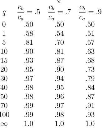
Assume thatcb 6ca. Using L’Hospital’s rule, π is seen to approach 1as

q goes to +_∞ and to approach 1

2 as q goes to 0. Table 1A presents select

values of π for alternative values of q andcb/ca =.5, .7 and .9.

In all cases π increases rapidly from .5 when q = 0 to levels larger than

.0 for values of q over 40. It is also seen that the rate of increase of π

is significantly lower for higher values of cb/ca (which make no-work more

π

q cb

ca

=.5 cb

ca

=.7 cb

ca

=.9

0 .50 .50 .50

1 .58 .54 .51

5 .81 .70 .57

10 .90 .81 .63

15 .93 .87 .68

20 .95 .90 .73

30 .97 .94 .79

40 .98 .95 .84

50 .98 .96 .87

70 .99 .97 .91

100 .99 .98 .93

∞ 1.0 1.0 1.0

Appendix B

Given the definition of pa, (22), ∂_∂p_caa =qpa(1−pa)u0(ca), ∂_∂cpa_a =−qpa(1−

pa)v0(cb)and∂_∂p_qa =pa(1−pa)(u(ca)−θ−v(cb)). By (23), totally differentiating

the optimum (bca,bcb)and pba w.r.t. q:

dcW(q)

dq =

∞

R

0

{[p_ba+ (u(bca)−θ−v(bcb))qpba(1−pba)]u0(bca)d_dqbca+

[(1_−bpa)−(u(cba)−θ−v(bcb))qpba(1−pba)]v0(bcb)d_dqbcb+

(u(_bca)−θ−v(bcb))2pa(1−pa)}dF(θ)

(B.1)

Differentiating totally the resource constraint, (24):

∞

R

0

{[pba+ (bca−1−bcb)qpba(1−pba)u0(cba)]d_dqbca+

[(1₋p_ba)−(bca−1−bcb)qpba(1−pba)v0(bcb)]d_dqbcb =

−R∞

0 b

pa(1−pba)(u(bca)−θ−v(bcb))}dF(θ)

(B.2)

Inserting (B.2) and the F.O.C. (14)-(15) in the paper into (B.1), we obtain

dWc(q)

dq =

∞

R

0 b

pa(1−pba)(u(cba)−θ−v(bcb))

[u(_bca)−θ−v(bcb)−bλ(bca−1−bcb)]dF(θ).

(B.3)

By (27), bλ > 0. Thus, at an interior optimum, an implicit positive tax

on work, 1−bca+bcb >0, implies

dWc(q)

References

[1] Anderson, S.P., A. de-Palma and J.F. Thisse (1992), Discrete Choice

Theory of Product Differentiation, (MIT Press).

[2] Diamond, P. and J. Mirrlees (1978), “A Model of Social Insurance with

Variable Retirement,”Journal of Public Economics, 10, 295-336.

[3] Diamond, P. and E. Sheshinski (1995), “Economic Aspects of Optimal

Disability Benefits,”Journal of Public Economics, 57, 1-23.

[4] Debreu, G. (1960) “Review of R.D. Luce, Individual Choice Behavior: A

Theoretical Analysis,”American Economic Review, 50, 186-188.

[5] Lowenstein, G. (2000), “Is More Choice Always Better?”, National

Academy of Social Insurance, (Social Security Brief).

[6] Luce, R.D. (1959) Individual Choice Behavior: A Theoretical Analysis

(Wiley).

[7] Mirrlees, J.A. (1987) “Economic Policy and Nonrational Behavior,” Uni-versity of California at Berkeley.

[8] Tversky, A. (1969) “Intransitivity and Preferences,” Psychological

Re-view, 76, 31-48.

[9] Tversky, A. (1972). “Elimination by Aspects: A Theory of Choice,”

0 θθθθ^ θθθθ

Figure 1

1/2 1

P_a

q = 0

q₀

q₁(>q₀)

W

W(q = ∞∞∞∞₎

W(q) ^ ^ q 0 ) ( ) 2 1 ( ) 0 (

ˆ _{q U R E} θ

W = = + −

) ( ) 1 (

ˆ _{U R E} θ

Wa = + −

) (R U W_b =

0 q

c

) (

ˆ q=∞

c_a 2 1 ) 0 ( ˆ ) 0 (

ˆ =c =R+

c_{a b}

) (

ˆ _q=∞

q 0

W

q₀

q₀ q

0 ) (

ˆ _q=∞

W

) ( ) 1

(_{R E} θ

U

Wa = + −

) (

ˆ q

W

) (R U W_b =

1

+ =R c_a

) (

ˆ _q=∞

ca

) (

ˆ _q=∞

cb

) (

ˆ q

c_a

) (

ˆ q