High Performance Novel Square Root Architecture Using Ancient Indian Mathematics for High Speed Signal Processing

http://dx.doi.org/10.4236/apm.2015.58042

High Performance Novel Square Root

Architecture Using Ancient Indian

Mathematics for High Speed

Signal Processing

Arindam Banerjee, Aniruddha Ghosh, Mainuck Das

Department of ECE, JIS College of Engineering, Kalyani, India

Email: banerjee.arindam1@gmail.com, ghoshani19@gmail.com, mrmainuckdas@gmail.com

Received 22 April 2015; accepted 8 June 2015; published June 2015

Copyright © 2015 by authors and Scientific Research Publishing Inc.

This work is licensed under the Creative Commons Attribution International License (CC BY).

http://creativecommons.org/licenses/by/4.0/

Abstract

Novel high speed energy efficient square root architecture has been reported in this paper. In this architecture, we have blended ancient Indian Vedic mathematics and Bakhshali mathematics to achieve a significant amount of accuracy in performing the square root operation. Basically, Vedic Duplex method and iterative division method reported in Bakhshali Manuscript have been utilized for that computation. The proposed technique has been compared with the well known Newton- Raphson’s (N-R) technique for square root computation. The algorithm has been implemented and tested using Modelsim simulator, and performance parameters such as the number of lookup tables, propagation delay and power consumption have been estimated using Xilinx ISE simulator. The functionality of the circuitry has been checked using Xilinx Virtex-5 FPGA board.

Keywords

Vedic Mathematics, Bakhshali Mathematics, Duplex, Yavadunam Sutra

1. Introduction

root computation so far. We are showing an efficient technique using ancient Indian mathematics.

In ancient times, mathematicians made calculations based on 16 Sutras (Formulae). The idea for designing the square root processor has been adopted from ancient Indian mathematics “Vedas” [10] [11]. The well known duplex method is an ancient Indian method of extracting the square root. The algorithm incorporates digit by di-git method for calculating the square root of a whole or decimal number one didi-git at a time. As per the proposed algorithm, the square root of any number is obtained in one step which reduces the iterations. Bakhshali method is used for finding a proximal square root described in ancient Indian mathematical manuscript called the Bakh-shali manuscript. A prototype of 16 bit square root processors has been implemented and their functionality has been experimented on a Virtex-5 FPGA board. For calculating integer part of a number, we have used the Vedic method and for calculating the floating point part, we have adopted Bakhshali method. Many researchers have used the most popular Newton-Raphson’s method for computing square root of a number. In our methodology, we are combining both Vedic duplex and Bakhshali approximation to generate more accurate result with com-paratively less time and power consumption.

The paper has been organized as follows. Section 2 describes the back ground mathematics for calculating the square root. Section 3 gives the architectural description of the proposed technique. Section 4 describes the error calculation and accuracy analysis of the proposed technique. Result analysis has been described in Section 5 and Section 6 is the conclusion.

2. Square Root Algorithm

Square root technique using Division method was introduced by ancient Indian Mathematicians and the proce-dure has been lucidly discussed in “Vedas”. The technique stands upon the execution by mere observation. Square root of a perfect square can be easily determined by the Division method. But for those numbers, which are not perfect square, Division method is not enough to compute with high precision. In this paper an iterative method described in Bakhshali Mathematics of Quran has been proposed to achieve high speed and high preci-sion square root calculation. The mathematical formulation of the iterative approach is shown below.

Consider a number X whose square root is to be calculated. The Bakhshali manuscript approach computes the square root of the perfect square which is nearest but less than the number X by the method of observational in-spection. Consider A is the above mentioned perfect square whose square root is R.

So it can be expressed as

2

X A Y R Y= ± = ± (1) where Y is the residue.

Equation (1) can be reformulated as

2 2 1 Y X R

R

 

= _ ± _

  (2)

So the square root of X can be written as

1 2 1 2

2 1 Y

X R

R

 

= _ ± _

  (3)

Using binomial expansion and the mathematical formulae of Bakhshali manuscript, Equation (3) can be ex-pressed as

2 3 4

1 2

2 2 2 2

1 1 1

1

8 16 32

2

Y Y Y Y

X R

R R R R

 _{     } 

≅  ± − _{ } ± _{ } − _{ } ± 

     

 

  (4)

2 3 4

2 2 2 2 2

1 1 1 1 1

1

2 2 2

2 2 2 2

Y Y Y Y

R

R R R R

R R R R R

 _{     } 

=  ± − _{ } ± × _{ } − × _{ } ± 

     

 

  (5)

2 2

2 12 2 2

1 1

2

2 2 2 2

Y Y Y Y

R

R

R R R R

 _{ } _{  } _

=  ± − _{  } +_{  }

   

  

2 1

2 2 2

1

1 1

2

2 2 2

Y Y Y

R

R

R R R

−

 _{   } 

=  ± − _{  } ± _ 

   

 

  (7)

2

2 2

2 2 1

2 _{2 1}

2

Y

Y R

R

Y

R _R

R

 _{ } 

 _ _ 

 

= ± −

  _± 

  

 

 

(8)

2

2 2

2 _{2 1}

2

Y

Y R

R

Y

R _R

R

 

 

 

= ± −

 _± 

 

 

(9)

2

2

2 ₂

2

Y

Y R

R

Y

R _R

R

 

 

 

= ± −

 _± 

 

 

(10)

Equation (10) is the modified Bakshali expression for computing the square root of non-squared numbers. In modified Bakshali approach the accuracy is more as comparable to in Bakshali approach which is shown in the table. So in respect of accuracy modified Bakshali approach is beneficial. Also Bakshali methodology con-tains some drawbacks mentioned below:

1) Bakshali approach does not gives the idea for computing the nearest squared number and its squareroot. To obtain thenearest square number and its square root we have to go for Vedic approach.

2) The division method for calculating the square root using Vedic mathematics is based on “Vilokanam” (Inspection) method which incorporates an extra squaring and extra subtraction operations.

The modified Bakshali approach eliminates the extra squaring and subtraction operations. thus the technique reduces the stage delay.

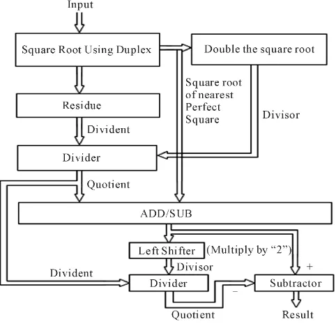
[image:3.595.193.434.470.704.2]

The square root determination technique combining the Vedic Duplex and Bakhshali approach is shown in the flow chart ofFigure 1.

2.1. Integral Square Root Determinant Using Vedic Methodology Mathematical Modeling of the Algorithm to Calculate Perfect Square Root Consider X is an N bit number whose square root is to be determined. X can be expressed as

1 1

0 2 2 2

2

1 2 2 0 2 0 2

N N

i i N i i

i i N i

N i i

X = x − x − x

+

− = =

=

∑

=

∑

+

∑

(11)

1 1 1

2 ₂ 2 _{2 2}

2

0 0 0

2 2

2N N 2 2i N N 2i N 2 ,i

i N N N i

i y i x_i y_i i x

− − − + = = _{+ +} =   = + _ − _ +  

∑

∑

∑

(12)

Considering 2 1 2 0 2 N i i N i y − + =

∑

to be the nearest perfect square number of 2 1 2 0 2 N i i N i x − + =

∑

. Now assume that the

square root of 2 1 2 0 2 N i i N i y − + =

∑

is 4 4 1

4 0

2N N 2i

i N i

Z =

∑

=− z+ . Then, Equation (12) can be rewritten as

1 1

2 2 4

4

0 0 ₁

2 2

2 4

0

2 2 2

2 2

2

N N N

i i

N N i n

i _{i i} i N

i i i

x y x

X Z Z x

Z − − + = _{+ +} = ₋ =     − +  _ _      = + _{ }+      

∑

∑

∑

(13)

Now consider

1 1

2 2 4

4

0 0

2 2

2 2 2

2 2

N N N

i i

N N i n

i x_i y_i i x _R

Q Z Z − − + = _{+ +} =     − +  _ _     _{= +}        

∑

∑

, (14)

where Q is the quotient and R is the remainder. Inserting Equation (14), Equation (13) can be reformulated as

1

2 4

0

2 N 2i

i i X Z= + ZQ+_R+ ₌− x _



∑

 (15)

Equation (15) can be rewritten as

(

)

1

2 2 ₄ 2

0

1

2 4 2

0 2 2 2 N i i i N i i i

X Z ZQ Q R x Q

Z Q R x Q

− = − =   = + + + + −      = + + + −   

∑

∑

(16)

Assume 4 1 2

0 2

N i i i

R+

∑

=− x −Q = p. Then X can be represented as,

(

)

2

X = Z Q+ +p (17)

(

)

(

)

(

)

2 2

2

1 p

X Z Q p Z Q

Z Q

 

 

= + + = + _ + _

+

  (18)

(

)

(

)

2

1 p Z Q Z Q     = + _ + _ +

(

_{) (}

₎

(

)

(

_{) (}

₎

2

2 2

2

2 p Z Q p

Z Q

Z Q _p

Z Q

Z Q

 

 

 ₊ 

 

= + ± −

+  

+ ±

 

 ₊ 

 

(20)

The procedure to calculate the square root by division method can be described in the following steps: Step 1: Obtain the nearest square root of the N/2 Most Significant Bits (MSB). Assume that the output is Z. Step 2: Determine the square of Z by combining Yavadunam and Duplex methodology.

Step 3: Subtract the squared output from N/2 MSB. Step 4: Obtain the double of Z.

Step 5: Combine the output of the subtractor and the next N/4 bits. Divide the combination by 2Z. Assume the quotient as Q and the remainder as R.

Step 6: Determine the square of Q and subtract Q2 from 4 1

0 2

N i i i

R+

∑

=− x . If the residue (p) is zero then X is the perfect square number whose square root is (Z + Q) otherwise (Z + Q) is the square root of the perfect square nearest to X. Again if “p” is positive then the nearest perfect square number is less than the given input else if “p” is negative then the nearest perfect square number is greater than the input.

Step 7: Compute

₍

₎

2

p

Z Q+ by Straight Division (“Dhvajanka”) methodology.

Step 8: Determine the square of

₍

₎

2

p Z Q+ .

Step 9: Compute

(

) (

₎

2

p Z Q

Z Q

 

+ ±

 

 ₊ 

  by add/sub unit.

Step 10: Finally subtract

(

)

(

_{) ( )}

2

2

2

2 p Z Q

p Z Q

Z Q

 

 

 ₊ 

 

 

+ ±

 

 ₊ 

 

from

(

) (

₎

2 p Z Q

Z Q

+ ±

+ to obtain the exact square root.

Step 11: Compute the maximum power of first left most “1” of

(

) ( )

(

)

(

_{) ( )}

2

2 2

2

2 p Z Q p

Z Q

Z Q _{Z Q} p

Z Q

 

 

 ₊ 

 

+ ± −

+  

+ ±

 

 ₊ 

 

by left shifting operation.

3. Proposed Architecture

Square Root architecture following the methodology given in Step 1 to Step 6, consists of four sub sections: 1) Nearest Square Root Generation Unit (NSRGU) for first N/2 numbers; 2) Squaring Unit; 3) Sub-tractor; 4) Di-vider.Figure 2 exhibits a fully optimized system level architecture for square root generation using Duplex me-thod adopted by ancient Indian mathematicians. In this architecture all the left shifters are N/4 bit left shifters. Quotient register is used to store the fixed point or integral result of the square root. The most significant two bits fed to the doubler whose output is fed to the subtraction unit.

3.1. Nearest Square Root Generation Unit

[image:6.595.170.458.82.380.2]

Figure 2. System level architecture for Integral part of Square root generator,

N indicating number of input bits.

must be of N/4 bits. The architecture of the nearest square root generation unit is same as the figure depicted in Figure 2. The above mentioned Step 1 to Step 6 are needed to obtain the nearest square root for N/2 bit number.

3.2. Squaring Unit

Squaring algorithm and the corresponding architecture was implemented with the aid of “Yavadunam Sutra”.

Mathematical Formulation of Yavadunam Sutra

If a number X is between 2n − 1 and 2n then the average of 2n − 1 and 2n is 2 1 2 _{3 2} 2 2

n n

n

A₌ − + _{= ×} − _{. If X > A}

then 2n is chosen as radix and if X A≤ then 2n − 1 is the selected radix. In Binary mathematics, the number n₀1 2i

i i

X − x

=

=

∑

can be reformulated as, 2

1

12 0 2, when adix 2 1R n

n i

n i i

X x − − x n

− =

= +

∑

= − (21)

(

)

2n 2 s complement of , when Radix 2

X = − ′ X = n (22)

From Equation (21), the square of the number X can be expressed as,

(

) (

2

)

₂

(

₂

)

2

2 1 1

12 2 12 0 2 0 2

n n

n n i i

n n i i i i

X x − x − − x − x

− − = =

= +

∑

+

∑

(23)

(

2

)

1

0

2n n 2i

i i

X − x

−

=

= +

∑

(24)

Similarly, the expression of X2 _{that can be obtained from Equation (22) is given as,}

(

) (

)

2

2 ₂n _{2 s complement of 2 s complement of}

Equation (24) and Equation (25) are the mathematical formulations of Yavadunam Sutra in Binary mathe-matics.

The architecture of squaring algorithm using “Yavadunam Sutra” is shown inFigure 3. The basic building blocks of the architecture are 1) RSU, 2) Subtractor, 3) Add-Sub unit and 4) Duplex squaring architecture. The test bench waveform of RSU is shown inFigure 4. The Subtractor architecture using “Nikhilam” sutra has been elucidated in sub-section-(C).

The input bits X (of length n) is fed to the RSU. The RSU produces proper radix and exponent for the input. The radix is subtracted from the input and the result is added to or subtracted from the input again depending upon the control signal generated from the borrow output of the sub-tractor. The output of add/sub unit is the re-sidue which is again squared by duplex operation discussed in [1] and it is also fed to the left shifter which shift the data depending upon the exponent value. Finally the outputs of duplex squarer and left shifter are added to obtain the squared result.

3.3. Subtractor

Mathematical Modeling of “Nikhilam” Sutra for Binary Subtraction

The Subtraction method has been implemented using normal binary arithmetic. It is a bit wise subtraction me-thod. The rule is mathematically expressed in Equation (26). Consider the number, n 1₁ 2i

i n

Y =

∑

−− y is to be sub-tracted from the number n₀1 2i

i i

[image:7.595.244.381.320.491.2]

X =

∑

=− x . So, it can be written as

[image:7.595.155.473.478.702.2]

Figure 3. Architecture of squaring al-gorithm using “Yavadunam” sutra.

(

)

1

0 2 2

n i i

i i

i

X Y− =

∑

₌− x −y (26) There is a borrow bit generated at the end of operation which signifies that the result is positive or negative.

3.4. Divider Using “Dhvajanka” Sutra (“On Top of the Flag”) 3.4.1. Mathematical Modeling of Division Operation

Consider the number n2 1₀ i i i

A −a x

=

=

∑

to be divided by n2 1₀ i i i

B −b x

=

=

∑

assuming that both the numbers are of same length (here the length is (n/2) − 1) and x is the radix. To execute the division operation easily and effi-ciently by “Dhvajanka” sutra (“On top of the flag”) methodology described in the ancient Indian Vedic Mathe-matics, Dividend must have greater length than Divisor. Consider again a number A' which can be represented

as 2 2 2 1 1

0 0 , 0,1,2, , ₂ 1 0

n n

n i n i

i i i

i i

n

A x A x −a x − a x a i

= =

    

= × = × = _∀ ∈_{  }− _=

 

 

 ′



∑

∑

. n2 1₀ i

i i

B=

∑

=−b x can be mapped

with 21

0 n

i i i

B′ =

∑

₌−b x′ where the condition of mapping is 0,1,2, , 1 2

i i n

b b i= ∀ ∈_  _{ }− _  

 

′ . The quotient Q can be

determined as

2

2 n

n

A A x A

Q x

B B B

₋ 

   

  _− _

′×  ′

′ ′

= = =_{ }×

  (27)

The term _x−2n_{, where x is the radix is to be extracted by Exponent Extraction Unit (EEU). In Binary number}

system, the radix “x” is equal to 2. Then from Equation (27), it is obvious that the result of A

B is needed to be shifted right by n/2 terms which has been shown inFigure 5, to get the actual quotient. The mathematical mod-eling of division operation by “Vertically and Crosswise” methodology has been described in the following subsection.

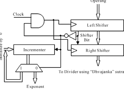
The architecture shown inFigure 6 consists of some elementary building blocks like left shifter, right shifter, incrementer and demultiplexer. Incrementer calculates the exponent of the number which is controlled by the shifted bit. The clock applied to the shifter is also controlled by the shifted bit. If the shifted bit is “1” then the shifters stops further shifting.

3.4.2. Mathematical Modeling of “On Top of the Flag” Sutra

Consider the number n₀1 i i i

A′=

∑

=−a x′ is divided by

1 2

0 n

i i i

[image:8.595.196.433.535.706.2]

B′ =

∑

=− b x′ . So A' can be expressed in terms of B' as

[image:9.595.170.461.83.303.2]

Figure 6. Divider architecture using “Dhvajanka” sutra.

1 1 2 3 4 3 2 1 0

1 2 3 4 3 2 1 0

0

n i n n n n

i n n n n

i

A − a x a x − a x − a x− a x − a x a x a x a x

− − − −

=

′=

∑

′ = ′ + ′ + ′ + ′ + + ′ + ′ + ′′ + ′ (28)

1 2 ₀

2 2

0

1 2

2 2

1

2 _{2 2}

2 2 1 2 1 3 ₃ 2 1 2 2 1 2 ₂ 2 1 ₁ 2

1 2 2

1 1

2 2

n n

n n

n

n n n

n n n n n n n n n n n n n n n

b x b x b x

a

a b b

b a a b b b a a b b

a _{x x}

b b − − − − − − _{− −} − − − ₋ − − − − ₋ − ₋ − − −   =_ + + + _           − ×       _{   }       −_{ } −     _{ }  ₋                 ′ ′ ′ ′ ′ ′ ′ ′ ′ ′ ′ ′ ′ ′ ′ ′ ′ ′ + ′ × + ′ 1 2 2 1 2 n n x b − −                                  _ _     ₊                        ′ (29)

[image:9.595.110.539.278.573.2]

Here “x” signifies the radix.

Figure 6shows the architectural description of division operation using “On top of the flag” Sutra. The Divi-dend of N bits is divided into two equal N/2 bits. The most significant part is fed to the subtractor which is of N/2 + 1 bits size. Single bit zero padding is done in subtractor module to the left. The division procedure incor-porated here is non-restoring type of division. The carry output after the subtraction is fed to the quotient array register as quotient.

The quotient array register stores the quotients based on the iterated value which is used as position signal. The value N/2 + 1 is stored in the decrementer initially to count and check the specified iteration. After each ite-ration, both the left shifters are updated by shifting until the decremented value reaches zero.

[image:10.595.173.447.84.348.2]

Figure 7. Divider architecture combining exponent extraction and “Dhva-janka” sutra.

sutra, 3) Subtractor, 4) Quotient Array Register and 5) Bidirectional Shift Register. Zero padding is needed to represent a number to higher number of bits. For example if a four bit number “0111” is represented in eight bit format then the representation becomes “00000111”. Here, zero padding has been executed based on the re-quirement. Bidirectional shift register performs the operation of shifting both to the left or right depending upon the control signal “carry” from the second subtractor. If carry = 0 then the input bits are shifted to the left and if carry = 1 then input bits are shifted to the right. The result of the second subtractor is fed to the shifter to control number shifting. The contents of the Quotient Array Register are the input to the Bidirectional Shift register.

Illustration: Consider a fourth order function

( )

3 2 1 0

3 2 1 0

f x =a x a x a x a x+ + + and a second order function

( )

1 0

1 0

g x =b x b x+ . We have to compute f x

( )

_{( )}

g x with the help of “On top of the flag” sutra. Now,

( )

( )

( )

( )

( )

( ) ( )

3 2 1 0

3 2 1 0

1 0

1 0

f x a x a x a x a x _{Q x} R _{f x Q x g x R}

g x b x b x g x

+ + +

= = + ⇒ = +

+

where,

( )

3

2 0

1

1 0

1 3

2 0

1

2 1 0

3

1 1 1

a

a b

b

a b

b a

a b

b a

Q x x x x

b b b

     

−

     

  ₋   

 _{ }   

 _ − _ _ _ 

 _{   } 

=_ + + _

 

 

 

 

 

 

and

3

2 0

1

1 0

1

0 0

1 a

a b

b

a b

b

R a b

b

   

−

   

 

 ₋ 

 

 

 

 

= −

3.4.3. Adder-Subtractor Unit Using “Nikhilam” Sutra for Subtraction

been designed with the help of well-known binary addition/subtraction methodology. The architecture of Adder- Subtractor unit is shown inFigure 8. The carry signal from the square root determinant shown inFigure 2 is fed to the adder-subtractor unit at the control pin to assign the type of operation (addition/subtraction). If the carry signal is low then addition operation is executed else subtraction operation is executed.

4. Error Calculation and Accuracy Analysis

The exact expression for square root can be recapitulated from Equation (3) as,

1 2 2 3 4 5

1 2

2 2 2 2 2 2

1 1 5 7

1 1

8 16 4 32 4 64

2

Y Y Y Y Y Y

X R R

R R R R R R

 

         

= _ ± _ =  ± − _ _ ± _ _ − _× _ _ ± _× _ _ − 

 

  (30)

The approximated expression for the square root can be expressed as,

2 3 4 5

1 2

2 2 2 2 2

1 1 1 1

1

8 16 32 64

2

Y Y Y Y Y

X R

R R R R R

 _{       } 

≅  ± − _{ } ± _{ } − _{ } ± _{ } − 

       

 

  (31)

So the computational error (ec) in determining the square root can be expressed as,

1

2 4 1

1 2

2 2

1 ₁ 1

32 2

c exact approximated Y Y

e X X R

R R

−

  _{    }

=_ − _≅ × _{  } ± _{ }     

  (32)

The percentage of error in calculating the square root is,

( )

1 4

2 2

1 2 2

4 4

2 2

1 2

2

2

2 2

1 ₁ 1

32 2

% 100

1

1 1

32 ₁₀₀ 32 ₁₀₀

1

1 ₁

1 1 ₂

2 c

Y Y

R

R R

e

Y R

R

Y Y

R R

Y

Y Y

R

R R

−

 _{    }   _{×    ±  }        

≅_{ }×

 _{ } 

±

 _ _ 

 

 

   

 

   

 _{ }  _{ }

= × < ×

 

_{    }  _±  

  

± × ±

 _ _ _ _  _{  }

 

 

[image:11.595.127.543.169.706.2]

(33)

If x Y₂ R

= , then can easily be shown that 4 ₂ 1 1 1 4 32 128 100 32 1

2 x

x < × = <

 ₋ 

 

 

.

So,

( )

1 4

2 2 4

1 2

2 2

1 ₁ 1

32 2 1

% 100 100 100 1%

100 32 1

1 ₂

c

Y Y

R

R R x

e

x Y

R R

−

 _{    }   _{×    ±  }        

≅_{ }× < × < × =

 

 _{ }  _{ − }

±

 _ _  _{ }

 

. It is obvious that

the error is minimum if and only if _X1 2_{=R that is if Y = 0. Putting Y = 0 in Equation (33), the expression} be-comes

( )

% 0 100 0%

1 c

e = _{ }× =

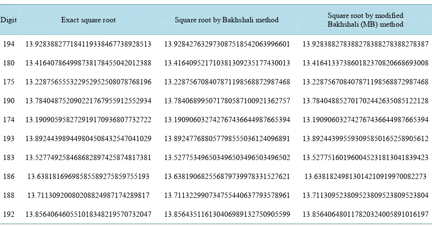
  .Table 1 exhibits the comparative study of the computational error in proposed

algorithm with respect to “Bakshali” algorithm.

5. Result Analysis

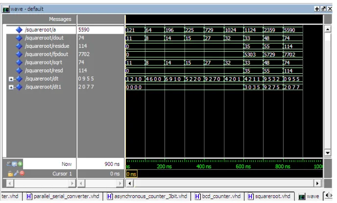
[image:12.595.90.535.370.603.2]

The square root architecture has been implemented using VHDL and verified using Modelsim simulator which is shown inFigure 9 and tested in Xilinx simulator with Xilinx Vertex-5 FPGA using XC5VLX30 device with a package FF676 at a speed grade (−3).Table 2 shows the comparative study of the N-R method and the proposed method with respect to LUT count, delay and power consumption. The power has been measured using Xilinx Xpower Analyzer tool.

Table 1. Coefficients of the quotient expression.

Digit Exact square root Square root by Bakhshali method Square root by modified _{Bakhshali (MB) method}

194 13.928388277184119338467738928513 13.928427632973087518542063996601 13.928388278388278388278388278387

180 13.416407864998738178455042012388 13.416409521710381309235177430013 13.416413373860182370820668693008

175 13.228756555322952952508078768196 13.228756708407871198568872987468 13.228756708407871198568872987468

190 13.784048752090221767955912552934 13.784068995071780587100921362757 13.784048852701702442635085122128

174 13.190905958272919170936807732722 13.190906032742767436644987665394 13.190906032742767436644987665394

193 13.892443989449804508432547041029 13.892477688057798555036124096891 13.892443995593095850165258905612

183 13.527749258468682897425874817381 13.527753496503496503496503496502 13.527751601960045231813041839423

186 13.63818169698585589275859755193 13.638190682556879739978331527621 13.63818249813014210919970082273

188 13.71130920080208824987174289817 13.711322990734755440637793578961 13.711309523809523809523809523804

[image:12.595.89.538.631.720.2]

192 13.856406460551018348219570732047 13.856435116130406989132750905599 13.856406480117820324005891016197

Table 2. Comparison of LUT count, delay and power of two methods.

Square root technique

4 bit 8 bit 16 bit

LUT (no.

of slices) Delay (ns) Power (mw) LUT (no. of slices) Delay (ns) Power (mw) LUT (no. of slices) Delay (ns) Power (mw)

N-R method 17 3.56 2.78 36 10.03 4.63 252 33.13 5.32

[image:13.595.144.488.82.290.2]

Figure 9. Test bench window of VHDL implementation of square root architecture.

6. Conclusion

From the result analysis, it is obvious that the architecture provides comparatively more accuracy than the well- known N-R approximation. Moreover, the proposed architecture produces less amount of propagation delay than N-R method and the power consumption is also very less as shown inTable 2. The area with respect to LUT count is also less than N-R method. It has also less circuit complexity than N-R technique which has been elucidated in the result analysis.

Acknowledgements

We would like to thank our dear colleagues for their precious support to execute the research in the department.

References

[1] Oberman, S.F. and Flynn, M.J. (1997) Design Issues in Division and Other Floating Point Operations. IEEE Transac-tions on Computers, 46, 154-161.

[2] Pineiro, J.A. and Bruguera, J.D. (2002) High-Speed Double-Precision Computation of Reciprocal, Division, Square Root, and Inverse Square Root. IEEE Transactions on Computers, 51, 1377-1388.

[3] Kwon, T.J. and Draper, J. (2008) Floating-Point Division and Square Root Implementation Using a Taylor-Series Ex-pansion Algorithm with Reduced Look-Up Tables. 51st Midwest Symposium on Circuits and Systems, Knoxville, 10- 13 August 2008, 954-995.

[4] Park, I. and Kim, T. (2009) Multiplier-Less and Table-Less Linear Approximation for Square and Square-Root. IEEE International Conference on Computer Design, Lake Tahoe, 4-7 October 2009, 378-383.

[5] Ramamoorthy, C., Goodman, J. and Kim, K. (1972) Some Properties of Iterative Square-Rooting Methods, Using High-speed Multiplication. IEEE Transaction on Computers, C-21, 837-847.

[6] Thakkar, A.J. and Ejnioui, A. (2006) Design and Implementation of Double Precision Floating Point Division and Square Root on FPGAs. IEEE Aerospace Conference, Big Sky.

[7] Ye, M., Liu, T., Ye, Y., Xu, G. and Xu, T. (2010) FPGA Implementation of CORDIC-Based Square Root Operation for Parameter Extraction of Digital Pre-Distortion for Power Amplifiers. 6th International Conference on Wireless Communications Networking and Mobile Computing, Chengdu, 23-25 September 2010, 1-4.

[8] Ercegovac, M.D. and McIlhenny, R. (2009) Design and FPGA Implementation of Radix-10 Algorithm for Square Root with Limited Precision Primitives. Conference Record of the Forty-Third Asilomar Conference on Signals, Systems and Computers, Pacific Grove, 1-4 November 2009, 935-939.

[10] Maharaja, B.K.T. (1994) Vedic Mathematics. Motilal Banarasidass Publisher, Delhi.