Fick’s Diffusion Experiments Revisited —Part I

http://dx.doi.org/10.4236/ahs.2014.34017

How to cite this paper: Patzek, T. W. (2014). Fick’s Diffusion Experiments Revisited—Part I. Advances in Historical Studies, 3, 194-206. http://dx.doi.org/10.4236/ahs.2014.34017

Fick’s Diffusion Experiments Revisited

—Part I

Tad W. Patzek

Department of Petroleum and Geosystems Engineering, The University of Texas, Austin, TX, USA Email: [email protected]

Received 25June 2014; revised 25July 2014; accepted 7August 2014

Copyright © 2014 by author and Scientific Research Publishing Inc.

This work is licensed under the Creative Commons Attribution International License (CC BY). http://creativecommons.org/licenses/by/4.0/

Abstract

In this paper, we revisit Fick’s original diffusion experiments and reconstruct the geometry of his inverted funnel. Part I demonstrates that Fick’s experimental approach was sound and measure-ments were accurate despite his own claims to the contrary. Using the standard modern approach, we predict Fick’s cylindrical tube measurements with a high degree of accuracy. We calculate that the salt reservoir at the bottom of the inverted funnel must have been about 5 cm in height and the unreported depth of the deepest salt concentration measurement by Fick was yet another 3 cm above the reservoir top. We verify the latter calculation by using Fick’s own calculated concentra-tion profiles and show that the modern diffusion theory predicts the inverted funnel measure-ments almost as well as those in the cylindrical tube. Part II is a translation of Fick’s discussion of diffusion in liquids in the first edition of his three-volume monograph on Medical Physics pub-lished in 1856, one year after his seminal Pogendorff Annalen paper On Diffusion.

Keywords

Salt Diffusion, Medical, Physics, Tube, Funnel, Experiment, Pogendorff Annalen

1. Introduction

195

brings interesting insights into Fick’s way of thinking about diffusion and osmosis, see Part II. The book section on the diffusion in liquids is more personal and somewhat different from the two famous papers published one year earlier (Fick, 1855a; Fick, 1855b).

This paper is a simple evaluation of Fick’s original experiments based on the theory of diffusion presented so well in (Hirschfelder et al., 1954) and (Bird et al., 1960). For an exquisite and brief discussion of the various theories of diffusion developed over the decades by Maxwell, Stefan, Onsager, Chapman and Enskog, Eckart and Meixner, and many others, one may refer to (Truesdell, 1962).

Fick’s theory of diffusion is almost as old as the theories of heat conduction by Fourier (Fourier, 1807; Fou-rier, 1822) and viscosity by Newton. While originally it was too primitive to reveal any ideas of principle, Maxwell soon1 gave it a rational basis in his kinetic theory of gas mixtures and Stefan (Stefan, 1871)cleared away the specifically kinetic details to achieve an inclusive phenomenological theory, see (Truesdell, 1966)for further details.

2. Background

For convenience, a few pertinent equations describing diffusion will be listed here. A full derivation may be found in, e.g., (Bird et al., 1960). Let vB denote the velocity of constituent

2_{B of a fluid mixture with respect to}

a stationary coordinate system, and define this velocity as by taking a snapshot of instantaneous velocities of the molecules of B. For a mixture of Nc constituents, we define the local mass-average velocity as

1 1

1

c c

c

N N

B B B B

B B

N

B B

ρ ρ

ρ ρ

= =

=

=

∑

=

∑

∑

v v

v (1)

Thus ρv is the local rate at which mass passes through a unit area perpendicular to v. Similarly, we may define a local molar average velocity as

* 1 1

1

c c

c

N N

B B B B

i B

N

B B

c c

c c

= =

=

=

∑

=

∑

∑

v v

v (2)

Thus cv* is the local rate at which moles pass through a unit area perpendicular to v*.

In flow systems one is often interested in the velocity of a given constituent with respect to v or v*, rather than with respect to a stationary coordinate system. This leads to the following definition of the diffusion veloci-ties:

( )

( )

* * *

diffusion velocity of relative to

diffusion velocity of relative to B

D B

B D B

B

B

≡ − =

≡ − =

v v v v

v v v v (3)

These velocities measure the motion of constituent B in a fluid relative to the local mean motion of the fluid. Now we can define the different mass and molar fluxes. The mass or molar flux of constituent B is defined as a vector whose magnitude is equal to the mass or moles of constituent B that pass through a unit area per unit time. The motion may be referred to stationary coordinates, to the local mass-average velocity, v, or to the lo-cal molar-average velocity, *

v . Thus the mass and molar flux densities relative to stationary coordinates are

( )m B =ρB B mass, ( )n B =cB B molar

j v j v (4)

The mass and molar flux densities relative to the mass-average velocity v are

( )m v B| =ρb ( )D B mass, ( )n v B| =cB ( )D B molar

j v j v (5)

and the mass and molar flux densities relative to the molar-average velocity v* are

1_{Maxwell published four important papers on gas theory, the first of which, “Illustrations of the Dynamical Theory of Gases”, appeared in}

1860, and contained Maxwell’s first theory of diffusion. See (Garber et al., 1986) for details.

196

( )

* ( )

_{( )}

* ( )

* *

| B D B mass, | B D B molar m v B =ρ n v B=c

j v j v (6)

Again, one should remember that the definition of a mass flux density is incomplete until both the units and the frame of reference are given.

By analogy with the flux of energy in one-dimensional systems:

(

)

d d

y p

q c T

y

α ρ

= − (Fourier’s law for constant

ρ

c_p), (7)

one may define the mass flux of constituent 1 in a binary system 12 as

( )

1 12 1

d d y

j D

y ρ

= − (Fourier’s law for constant ρ) (8)

Note that the total mass density, ρ, of the mixture is uniform, i.e., constant given a constant temperature. Here

α

is the thermal diffusivity, c_p is the heat capacity, D₁₂ is the diffusion coefficient, and

ρ

₁ is the mass density of constituent 1.

If the fluid density is not uniform, one defines the mass diffusivity D₁₂ =D₂₁ in a binary system in an analogous fashion:

( )m v| 1 12 1 mass,

_{( )}

_{n v|}*₁ 12 1 molar

j =ρD ∇w j =cD ∇x (9)

Note that Equation (9) is purely kinematic, i.e., it involves only the dimensions of length and time, and it must be justified from an independent dynamic theory that invokes forces.

It may easily be shown (Bird et al., 1960)that the mass or molar diffusion fluxes in Equation (9) are also given by

( ) ( ) ( )

( )

* ( ) ( )

2

1 12 1

| 1 1

1 2

1 12 1

1 | 1

1

m v m m B

B

n n B

n v

B

w D w

x cD x

ρ =

=

= − = − ∇

= − = − ∇

∑

∑

j j j

j j j

(10)

These two relationships are of special importance for this paper.

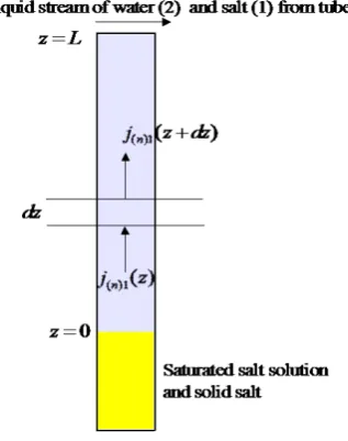
[image:3.595.237.396.481.682.2]

Fick’s experiment (Fick, 1855b)in a cylindrical tube is shown in Figure 1. At z=L, salt (1) diffuses into fresh water (2), while solid salt in a salt reservoir dissolves, replenishing the diffusing salt, and maintaining the

saturated salt concentration at z=0. A stream of fresh water sweeps the salt emerging from the tube, keeping the zero salt concentration at z=L. The whole system is at constant (albeit unknown) temperature and pressure. The mixture of salt and water is assumed ideal, i.e., each component activity is equal to its mole fraction.

When this dissolving salt system attains a steady state, there is a net motion of salt away from the salt reser-voir and the water in the tube is stationary. Hence we can use expression (10)2 for the molar flux of salt relative

to a stationary frame of reference:

( )

( )

( )

( )

( )

( )

( )

* 1 1 1 1 12 1

| 1

12 1 1

1

0

d ( )

1 d

n n

n v

n

j z j z x j z x cD x

cD x

j z

x z

= − − = − ∇

= − −

(11)

The salt mass balance over an incremental column height, dz states that at steady state

( )1

( )

d

0 d n

j z

z = (12)

Substitution of Equation (11) into Equation (12) gives

12 1

1 d d

0

d 1 d

cD x

z x z

 

=

 ₋ 

  (13)

We shall assume that D12 is nearly independent of concentration. Indeed the literature data show that D12≈ 1

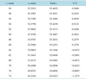
cm2/day for 0.1 - 1 normal salt solutions. The saturated salt concentration is about 36 g NaCl/100g of water or 26 g NaCl/100g solution at room temperatures of 10 - 20 degrees C. From Appendix, we can calculate the total concentration of water and salt at 20 deg C. This calculation is summarized in Table 1. The percent coefficient of variation is generally less than 1%; therefore, the total concentration can be assumed constant.

The coefficient of variation is defined as C.V. c c 100%

c − =

[image:4.595.173.453.458.716.2]

Thus, we can recast the steady state diffusion mass balance of salt, Equation (13), as

Table 1. Total concentration of aqueous salt solutions, see Appendix.

c1-water c5-water Total c C.V.

99 55.2915 55.4635 0.5408

98 55.1087 55.4551 0.5255

96 54.7360 55.4386 0.4956

94 54.3790 55.4478 0.5123

92 53.9682 55.4133 0.4498

90 53.5350 55.3667 0.3653

88 53.0787 55.3075 0.2579

86 52.5986 55.2353 0.1270

84 52.0893 55.1446 −0.0372

82 51.5643 55.0498 −0.2091

80 51.0133 54.9405 −0.4072

78 50.4400 54.8208 −0.6243

76 49.8391 54.6856 −0.8693

198

( )

( )

1

1

1 1

d

d 1

0

d 1 d

0 0.0976, 0

x

z x z

x x L

 

=

 ₋ 

 

= =

(14)

This equation can be easily solved (Bird et al., 1960) and the result is

( )

1 1

( )

( )

1 1

1 1

1 0 1 0

z L

x L x

x x

 − 

−

= _ _

− _ − _ (15)

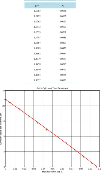
The density-mole concentration data from Table 1 and Table 2 are summarized in Table 3. The latter table can be used in conjunction with the excess gravities reported by Fick to convert his gravity versus depth results into the salt mole fraction versus depth. This was implemented as linear interpolation.

The results are shown in Figure 2. Agreement between the theory and experiment is excellent.

Remarks

Figure 3 shows the profile of excess gravity that would have been calculated by Fick for the cylindrical tube experiment. Note that there is a systematic deviation of the calculation from the experimental data. Fick himself said (Fick, 1855a): “That the degrees of concentration in the lower layers decrease a little more slowly than in the upper ones, is easily explained by the consideration, that the stationary condition had not been perfectly at-tained”. Similar excuses have been used by experimentalists ever since.

3. Fick’s Conical Funnel Experiment

[image:5.595.171.453.414.661.2]

The conical funnel data obtained by Fick (Fick, 1855a)are more difficult to decipher because of the incomplete reporting of the experiment. The most likely experiment geometry may be inferred from Figure 6. In an inverted

Table 2. Density and concentrations of aqueous NaCl solutions at 20 deg C. c1%

20 4 g/l

ρ δ c3 c5

1 1005.3 0.22 10.053 0.1720

2 1012.2 0.24 20.250 0.3464

4 1026.3 0.28 41.072 0.7026

6 1041.3 0.31 62.478 1.0688

8 1055.9 0.34 84.472 1.4451

10 1070.7 0.37 107.070 1.8317

12 1085.7 0.39 130.284 2.2288

14 1100.9 0.42 154.128 2.6367

16 1116.2 0.44 178.592 3.0553

18 1131.9 0.47 203.742 3.4855

20 1147.8 0.49 229.560 3.9272

22 1164.0 0.51 256.080 4.3808

24 1180.4 0.53 283.296 4.8465

26 1197.2 0.55 311.272 5.3251

The concentration units are explained above. The correction δ is as follows: if the solution density is determined at the temperature T1 in deg C, then one adds δ(T2−T1) to this density to

[image:6.595.145.483.103.682.2]

Table 3. Salt solution density at 20 deg C and the mole fraction of salt.

g/cc x1

1.0053 0.0031

1.0122 0.0062

1.0263 0.0127

1.0413 0.0193

1.0559 0.0261

1.0707 0.0331

1.0857 0.0403

1.1009 0.0477

1.1162 0.0554

1.1319 0.0633

1.1478 0.0715

1.1640 0.0799

1.1804 0.0886

1.1972 0.0976

Figure 2.Fick’s cylindrical tube excess gravities (+) have been converted to mole fractions of salt versus depth by linear interpolation of data inTable 3. The theoretical curve given by Equation (15) is the solid line. Note excellent agreement between theory and experiment.

0 0.01 0.02 0.03 0.04 0.05 0.06 0.07 0.08 0.09 0.1

0 5 10 15 20 25

Fick's Cylindrical Tube Experiment

E

lev

at

ion

abov

e s

a

lt r

es

er

voi

r,

c

m

Mole fraction of salt, x

[image:7.595.145.481.84.362.2]

200

Figure 3. This is how Fick would interpret his cylindrical tube experiment. Note the system-atic deviation between the data and the straight line drawn by Fick.

conical funnel, and in the absence of gravity, the salt concentration contours would be sections of concentric spheres centered on the salt reservoir at the funnel tip. One may argue that in the gravitational field the spherical concentration profiles of salt will be flattened vigorously by buoyancy force3. The denser salt solution near the funnel axis will sink, while the less dense solution near the walls will be buoyed. The concentration profiles will then become almost perfectly horizontal. With help of Figure 4, this assertion can be proven as follows. For the salt profile flattening to happen, the ratio of the characteristic time of diffusion,

τ

_D spreading the salt radially, and convection,

τ

_C, tumbling the more concentrated salt solution down a “hill” of height h, must be much more than one:

Fick’s Number Fi D 1 C

τ

τ

= _ , (16)

i.e., buoyancy flattens the constant salt concentration profiles before diffusion propagates them as sections of concentric spheres.

The characteristic diffusion time scale can be obtained from the diffusion coefficient, D12, and the distance, h:

2

12 D

h D

τ ≈ (17)

Assuming no viscous dissipation, the shortest convection time scale can be obtained from the balance of po-tential and kinetic energy:

2 ,max

,max

,max

1 2 2

2 C

C

C C

gh v

v gh

L v

ρ ρ

ρ ρ

τ

∆ =

≈ ∆

≈

(18)

0 0.02 0.04 0.06 0.08 0.1 0.12 0.14 0.16 0.18 0.2

0 5 10 15 20 25

Fick's Cylindrical Tube Experiment

E

lev

at

ion

abov

e s

a

lt r

es

er

voi

r,

c

m

Excess gravity, g/cc

Figure 4. Geometry of flattening of diffusion front.

From elementary geometry, it also follows that

(

)

sin , 1 cos L r h r α α =

= − (19)

By combining Equations (16)-(19), one obtains the following criterion

(

)

(

)

5 2 3 2 2 12 12 3 2 12 5

1 cos 2

Fi 1,

2 sin

2 2

2 sin

2 1 cos crit

r g

h D

g g

D

L g h

D r r g α ρ α ρ α α ′ − _′ ∆ ≈ = ≡ ′     ≡  _{′ −}      (20)

[image:8.595.203.525.84.487.2] [image:8.595.230.395.88.307.2]

The plot of the critical distance from the salt reservoir with the most conservative g′ =0.01g is given in Figure 5. It is obvious that at distances of more than 1 mm above the salt reservoir, the salt concentration pro-files are essentially flat.

The geometry of Fick’s cemented funnel experiments is shown in Figure 6. The junction between the funnel and the salt reservoir is at an unknown elevation z1 at which the salt solution is saturated. Because the deepest

reported salt density is far from the density of the saturated salt solution, there is an unknown offset δz be-tween z1 and the deepest measurement.

In the cylindrical-polar coordinate system in Figure 6, the vertical diffusion flux is

( )

( )

( )

( )

( )

( )

( )

( )

* 1 1 1 1 12 1

| 1 12 1 1 1 0 d 1 d n n n v n

j z j z x j z x cD x

cD x j z x z = − − = − ∇ = − − (21)

The salt mass balance over a cylinder with the base of πr2

( )

z and height dz, states that at steady state

( )

( )

( )

(

)

( )

( )

(

)

2 1 2 1 d 0, d d 0. d n n

r z j z

z

z j z

z

=

=

[image:9.595.141.483.88.366.2]

202

Figure 5. The critical distance from the salt reservoir at the tip of an inverted conical funnel versus the funnel half-angle. At distances much greater than the critical distance, the salt concentration profiles will be essentially flat.

Figure 6. Geometry of Fick’s funnel experi-ment.

Substitution of Equation (21) into Equation (22) and assumption of constant cD₁₂ give

( )

( )

2 1

1

1 1 1 2

d

d 1

0,

d 1 d

0.0976, 0.

x z

z x z

x z x z

 

=

 ₋ 

 

= =

(23)

Equation (23) can be readily solved (Bird et al., 1960) and the result is

5 10 15 20 25 30

10-5 10-4 10-3 10-2

Funnel half-angle, degrees

C

ri

ti

c

al

di

s

tanc

e,

c

[image:9.595.229.398.409.614.2]

( )

( )

( )

( )

1 1 2

1 1

1 1

1 1 2

1 1 1 1

1 1

1 1

z z z z

x z x z

x z x z

− −

 

− −

= _ _

− _ − _ (24)

To match Fick’s results with the theoretical curve (24), one needs to find the lower elevation z1 and the

measurement offset δz. Then z₂= +z₁ δz+

(

155.4 27.7 10 cm−

)

. The resulting two-parameter optimization problem has been solved using the Nelder-Mead amoeba algorithm and the solution is:

1

2

4.985 5 cm, 3.0848 3 cm, 20.84 21 cm.

z z z

δ

= ≈

= ≈

= ≈

(25)

Without invoking a nonzero offset, Fick’s experimental results cannot be matched. Thus, the funnel-salt res-ervoir junction corresponds to the elevation of 5 cm above the funnel tip and the deepest gravity measurement was preformed 3 cm above that junction. The resulting fit of Fick’s funnel data is shown in Figure 7. A little bit of scientific sleuthing has resulted in excellent agreement with Fick’s experimental data—a handsome reward indeed!

4. Discussion of Fick’s Equation

On no basis beyond an asserted analogy to Fourier’s analysis of the flow of heat, Fick proposed that in a binary mixture the diffusion mass flux density vector is proportional to the gradient of mass density:

( )m v B| B ( )D B B, 1, 2, 0,

j ≡ρ v = − ∇D ρ B= D> (26)

[image:10.595.146.482.403.683.2]

where D is a phenomenological coefficient which may depend upon the densities and the temperature. From Equation (9) we now know that Equation (26) holds only if the solution density is constant:

Figure 7. Fick’s conical funnel excess gravities (+) have been converted to mole fractions of salt versus by linear interpolation of data inTable 3. The theoretical curve given by Equation (24) is the solid line. Note excellent agreement between the theory and Fick’s experiment.

0 0.005 0.01 0.015 0.02 0.025 0.03 0.035 0.04 0.045 0.05

8 10 12 14 16 18 20 22

Fick's Conical Funnel Experiment

R

adi

al

di

s

tanc

e f

ro

m

s

al

t r

es

er

v

oi

r,

c

m

Mole fraction of salt, x

204

( ) ( )

(

)

( )

(

)

| ,

1 salt , 2 water , 0, const

B B B B

m v B D B

j D w D D

B B D

ρ ρ ρ ρ ρ ρ

ρ

≡ = − ∇ = − ∇ = − ∇

= = > =

v

(27)

Because densities of Fick’s salt solutions varied by 20%, Fick in fact was mistaken in asserting Equation (26). His subsequent diffusion equation was derived from a shell mass balance between two horizontal planes dz

apart.

Based on the mass balance shown in Figure 6, Fick derived the following equation:

( )

_{( )}

( ) ( )

_{( )}

(

) (

)

( )

(

( )

( )

( )

)

1 1 1 1 1

d , d , d

1

,

m m

m

A z z j z t A z j z z t A z z

t

A z j z t

t A z z

ρ ρ ∂ _{= + + +} ∂ ∂ _{= −} ∂ ∂ ∂ (28)

Instead of inserting the salt mass flux density from Equation (10) (he did not know this equation), Fick as-serted Equation (26), and obtained the following equation:

( )

2

1 1 1

2

1 d d

A D

t z A z z z

ρ  ρ ρ 

∂ ₌ ∂ ₊ ∂

 

 

∂ _ ∂ ∂ _. (29)

At steady state, and in the conical funnel whose radius is given as r z

( ) (

= tanα

)

z, Fick simplified Equation (29) and solved it:

( )

2 1 1 2 2 1 1

d 2d

0 d d , z z z C z C z ρ ρ ρ + = = − (30)

The two constants C₁ and C₂ “… are to be so determined, that for a certain z (where the cone is cut off and rests upon the salt reservoir4)

ρ

₁ is equal to perfect saturation; and for a certain value of z which corresponds to the base of the funnel5,

ρ

₁ becomes = 0”. Thus

(

)

(

)

1 z z2 0, 1 z z1 sat 0.196 g cc.

ρ = = ρ = =ρ = (31)

If Fick knew about Equation (10), then instead of Equation (30) he would have probably written:

( )

1 2 1

1 1

d d

d 1 d 1

0,

d 1 d d 1 d

x x

cD A z z

z x z z x z

   

= =

 ₋   ₋ 

    (32)

and he would have obtained Equation (23).

Because Fick does not report these “certain values of z”, to obtain the two constants we must use the elevation of the funnel base, and the offset of the deepest measurement calculated above. The two constants in Equation (30) are then readily calculated as C1= −0.0616,C2=1.2843. In the paper, however, Fick lists his calculated

salt density profile! The raw data, Fick’s calculation and the present calculation are shown in Figure 8. Agree-ment between the reconstructed solution and Fick’s “exact” calculation is very good indeed. The latter com-parison confirms validity of the elevations (or axial distances) listed in Equation (25). Of course, because of the incorrect form of the governing equation, the solutions shown in Figure 8 are nowhere nearly as good as the so-lution shown in Figure 7.

5. Conclusion

In general, Fick’s Equation (29) is not entirely correct. For the concentrated salt solutions, one may not assert that mass density

ρ

1 is the appropriate unit of concentration, and that ρ=const. As it stands, after the sign

correction, Fick’s original equation can only be applied to dilute solutions and to such tubes of variable cross- section whose walls are orthogonal to the surfaces of constant concentration. This does not detract however from

4_{Fick used y instead of} ρ

1 and x instead of z. So his “certain distance x” becomes z = z1 in our notation. 5_{Equal to the outer elevation z}

[image:12.595.147.483.86.368.2]

205

Figure 8. Fick’s excess gravity data (+) in the conical funnel, his calculated salt density pro-file (upper curve), and the propro-file reconstructed here with use of the previously obtained values of z1 and δz.

Fick’s great physical insight, and from his creative and quite accurate6 experimental technique!

Acknowledgements

I thank Ms. Karin Lloyd-Mumford for her patience and tenacity in translating Fick’s difficult prose. I am grate-ful to the late Prof. T. N. Narasimhan for sharing his insights into the theories of diffusion and copies of the out-of-print books and papers.

References

Achmatowicz, O. et al. (Ed.) (1954a). Chemical Calendar. Vol. I. Warsaw: PWN. (in Polish) Achmatowicz, O. et al. (Ed.) (1954b). Chemical Calendar.Vol. 2, Part II. Warsaw: PWN. (in Polish)

Bird, R. B., Stewart, W. E., & Lightfoot, E. N. (1960). Transport Phenomena. New York: John Wiley & Sons, Inc.

Fick, A. (1855a). On Liquid Diffusion. The London, Edinburgh, and Dublin Philosophical Magazine and Journal of Science, 10, 30-39.

Fick, A. (1855b). Ueber Diffusion (On Diffusion). Annalen der Physik und Chemie von J. C. Pogendorff, 94, 59-86. Fourier, J. B. J. (1807). Théorie des mouvements de la chaleur dans le corps solides. French Academy.

Fourier, J. B. J. (1822). Theory of Heat (Théorie Analytique del la Chaleur). Paris: F. Didot.

Garber, E., Brush, S. G., & Everitt, C. W. F. (Eds.) (1986). Maxwell on Molecules and Gases. Cambridge, Massachusetts: MIT Press.

Hirschfelder, J. O., Curtiss, C. F., & Bird, R. B. (1954). Molecular Theory of Gases and Liquids. New York: John Wiley & Sons, Inc.

Stefan, J. (1871). Über das Gleichgewicht und die Bewegung, insbesondere die Diffusion von Gasmengen. Wiener Sitzungs-

0 0.02 0.04 0.06 0.08 0.1 0.12

8 10 12 14 16 18 20 22

Fick's Conical Funnel Experiment

E

lev

at

ion ov

er

c

on

e t

ip,

c

m

Excess gravity, g/cc

Fick's data Fick's calculation TWP's calculation with r

1 and δr

6_{Fick remained modest about his approach: “… This method (of weighing an immersed glass bulb to determine density) creates little}

206

berichte, 63, 63-124.

Truesdell, C. (1962). Mechanical Basis of Diffusion. The Journal of Chemical Physics, 37.

Truesdell, C. (1966). The Elements of Continuum Mechanics. New York: Springer-Verlag.

Appendix—Different Units for Salt Concentrations

There are several ways of expressing salt concentrations (Achmatowicz et al., 1954a, 1954b): 1) Number of grams of salt per 100 g of solution, c1;

2) Number of grams of salt per 100 g of water, c2;

3) Number of grams of salt per 1 liter of solution, mass concentration, c3;

4) Number of moles of salt per 1000 moles of water, c4;

5) Number of moles of salt per 1 liter of solution, molar concentration, c5;

6) Number of moles of salt per 1 kg of water, molality, c6;

7) Mole fraction of salt in water, c7;

Let γ denote the specific gravity of solution, and M the molecular weight of salt:

3 2 3

1

2

3 6

1 2

1 3

2

3 1 5

2

2 4

3 1

5

2 6

4 7

4 100

10 100 10

100 100

100 1000 10

1000 10

100

180.2

10

10

1000

c c c M

c

c

c c M

c c

c c

c

c c c M

c c c

M

c c

c

M M

c c

M c c

c

γ γ

γ γ γ

γ

= = =

+

= = =

− −

= = =

+

=

= =

=

= +