Decoupled Sliding Mode Control for a Multivariable Nonlinear System

Decoupled Sliding Mode Control for a Multivariable

Nonlinear System

Fayez G. Areed

Prof.of Automatic Control Mansoura Univ. Faculty of Eng.

Computers & Systems Dep.

Mohamed A. Badr

Prof. of Automatic Control Ain Shans Univ. Faculty of Eng.

Electrical Engineering Dep.

Sabry F. Saraya

Ass. Prof. of Automatic Control Mansoura Univ. Faculty of Eng. Computers & Systems Dep.

Mohammed S. Elksasy

Dr. of Automatic Control Mansoura Univ. Faculty of Eng.

Computers & Systems Dep.

Mohamed M. Abdelsalam

M.SC of Automatic Control Mansoura Univ. Faculty of Eng.

Computers & Systems Dep

ABSTRACT

This paper presents a decoupled control strategy using time-varying sliding surface-based Sliding Mode Controller (SMC) for a multivariable nonlinear system as an Ammonia Reactor system. The decoupled method provides a simple way to achieve asymptotic stability by dividing the system into three subsystems. Simulation results are presented for SMC comparing with a traditional PID controller. Then , the system is subjected to temperature disturbance to demonstrate the effectiveness and robustness of the controller.

General Terms

Decoupled Sliding Mode Control.

Keywords

Sliding Mode Controller; Ammonia Reactor; Decoupled system; PID controller.

1.

INTRODUCTION

Sliding mode control provides (i) insensitivity to parameter variations; (ii) external disturbance rejection; and (iii) fast dynamic responses. These robust properties make this discontinuous control strategy very attractive [1-4].

The main idea of sliding mode control is to steer the system trajectories into the sliding surface and then keep them on it. So the control law consists of two parts: a continuous control which controls the system when its states are on the sliding plane and a discontinuous control which handles the uncertainties. In practice, the system states do not remain on the sliding surface after reaching it due to uncertainties in dynamical equations. Around the surface S, is often irritated by high frequency oscillations known as chattering [5-6]. The development of general sliding mode design approaches for multi-input nonlinear systems has been hampered by the need to reduce the nonlinear system to regular form [7-10]. Research on multivariable nonlinear systems with internal parameter uncertainties and external disturbances is important for both theoretical and practical reasons [11-13].

In this paper, a Decoupled Sliding Mode Controller (DSMC) design is used to control an Ammonia Reactor. The Reactor is divided into three subsystems with different switching surfaces. Comparing the DSMC controller with a traditional PID controller with exposing the system to temperature disturbance to demonstrate the effectiveness and robustness of the controller.

2.

SYSTEM DESCRIPTION

Ammonia synthesis is the first stage in the manufacturing of nitrous chemical products. In order to determine the optimum working regimes. This is determined by:

a. The direct synthesis reaction N2 + H2 ↔ NH3 is a reversible exothermic reaction which must take place at equilibrium to get a maximum conversion rate.

b. The conversion rate depends on: temperature (the temperature increase leads to ammonia decomposition, thus leading to conversion rate decrease), catalyst activity and pressure.

c. The synthesis columns are built with multiple fixed catalyst layers and Quenches to reduce the temperature and ammonia concentration at the input into the next layer d. The catalyst is spent non-uniform, starting with the first layer.

3.

AMMONIA REACTOR

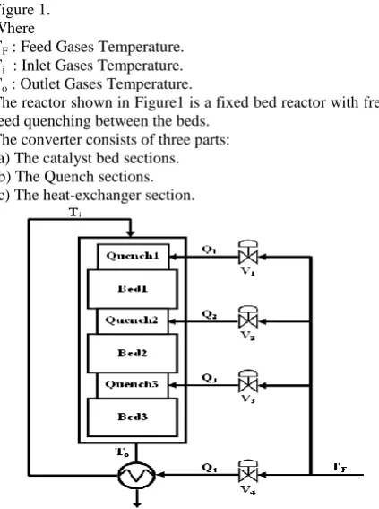
The ammonia reactor is the heart of the synthesis plant. Ammonia reactor with a fixed-bed quench cooling is shown in Figure 1.

Where

TF : Feed Gases Temperature.

Ti : Inlet Gases Temperature.

To : Outlet Gases Temperature.

The reactor shown in Figure1 is a fixed bed reactor with fresh feed quenching between the beds.

The converter consists of three parts:

(a) The catalyst bed sections. (b) The Quench sections.

Fig 1: Ammonia Reactor with Bed and Quenching Sections

The inlet gaseous mixture is split into four separate streams as:

(a) The main stream called the heat exchanger Flow (Q4). (b) The second stream which enters 1st Quench (Q1). (c) The third stream which enters 2nd Quench (Q2). (d) The Fourth stream which enters 3rd Quench (Q3)[14].

4.

MATHEMATICAL MODEL

4.1

Reactor Mathematical Model

The mathematical model of the ammonia reactor consists of one model for each bed. Each bed is described by a mass and

energy balance, and is discretized into ten segments [14].

) , (T c r m z c Q_  c



2 2

) , ( ) (

z T C m c T r m H z

T QC t T C

mc pc pg rx c c pc_

   

     



(2)

Where

t Time [sec.]

z Position in reactor.

T Particle temperature [K]

c Concentration of ammonia [kg NH3/kg gas] −Δ Hrx Heat of reaction [J/kg.NH3] Cpc Heat capacity of catalyst [J/kg cat.K]

Cpg Heat capacity of gas [J/kg.K]

mc Catalyst mass in the bed [Kg]

Q Gas flow through the bed [Kg/s]

r(T, c) Reaction rate [kg.NH3/kg cat.sec.] Γ Dispersion coefficient [1/sec]

The model may be discretized in space. So, the model can be rewritten in discretized equations for cell no. j as :

) , ( ) (

0Qcj1cj mc,jrTj cj ₍₃₎

) , ( ) ( )

( 1 ,

, pg j j rx cj j j

i pc j

c QC T T H m rT c

t T C

m    

 



(4) Hence each bed is descretized into 10 cells, so 30 equations describe the reactor model.

4.2

The Quench Model

Fresh feed quenching of the ammonia concentration are entering the reactor between each bed. Quenches are modeled as follows:

q q b

q b q b

b

mix T

Q Q

Q T Q Q

Q T

   

(5)

q q b

q b q b

b

mix c

Q Q

Q c Q Q

Q c

   

(6)

The subscript q, b and mix refer to the quench stream. The reactor flow before the quench and the reactor flow after the quench, respectively. Temperature, concentration of ammonia and mass flow are denoted T, c and Q.

4.3

The Heat Exchanger Model

The model of the heat exchanger as follows:

Ti = Є To+ (1-Є) TF (7)

Where Є is the heat exchanger efficiency

5.

OPEN LOOP SIMULATUIN RESULTS

From the reactor construction, inputs and outputs can be summarized as:

Reactor Inputs : The split Mass Flows enter the reactor (Q1,Q2,Q3,Q4) , Feed temperature of gasses. (TF), Feed

ammonia mass fraction(CF) and Feed pressure (P).

Reactor Outputs : Outlet gasses temperature (To) and outlet

ammonia mass fraction (Co).

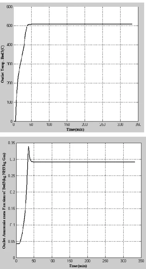
Fig 2: Reactor Outlet Temperature and Concentration.

reach the nominal value for beginning of conversion, so, a transient ammonia concentration is obtained. Till the temperature is stabilized and a stable reaction rate was obtained. The experts are not worry about the peak because of they prefer high outlet ammonia concentrations as commercial considerations.

6.

FEED TEMPERATURE

DISTURBANCE

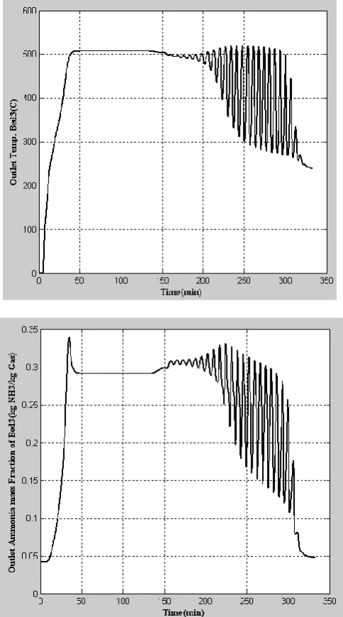
The feed temperature has been disturbed to 210°C , i.e., for about 30% from the regular Feed temperature. The outlet temperature and ammonia concentration due to the temperature disturbance are shown in Figure 3.

Fig 3: Disturbed Outlet Temperature and concentration.

Figure 3 shows high temperature oscillations after the temperature has been reduced to 210°C. These vibrations resumed for about 130 minutes then, the system stabilizes at 238.7°C. This means that the temperature is reduced by about 53% from its steady state stable value. High oscillations similar to the temperature and the system stabilizes at

ammonia concentration about 4.78% . i.e., the concentration reduced to about 83.75% from its steady state stable value.

7.

AMMONIA REACTOR

CONTROLLER DESIGN

Some issues have to be mentioned before embarking on the control of the ammonia reactor.

Firstly, the ammonia reactor operating point possesses the highest temperature, which leads to the highest conversion of ammonia, although it results in a lower yield of ammonia [15-17].

Secondly, the oscillations given in Figure 3 appeared as a result of too low inlet temperature through the ammonia reactor. To avoid the instability, one can naturally increase the inlet temperature, TF, or the reactor pressure (P), which may

be no suitable for the ammonia production unit. Another possibility is to increase the heat recovery by reducing the flows through the other quenches (Q1, Q2, Q3) so that more of

the feed is preheated [18-19]. The reactor system could be stabilized using the mass flow trough the quenches to control the temperatures at the inlet to the beds. This means using the temperature feed mass flow Q1 , Q2 and Q3 as manipulated

variables and the reactor inlet temperatures (after the quenches) as measurements. The block diagram of the controller as shown in Figure 4.

Where

Tb1ref, Tb2ref and Tb3ref : The Reference descretized Bed cells

temperatures.

Tb1, Tb2 and Tb2 : The Real descretized Bed cells

temperatures.

u1, u2 and u3 : The Valves control signals.

Q1, Q2 and Q3 : The mass flows enter the Quenches.

Tout : The Outlet Reactor temperature

Cout : The Outlet ammonia mass

concentration.

Fig 4: Block Diagram of Ammonia Reactor Controller

The control signal can vary as :

1

0u (8) where

u=1 the valve is fully opened and u=0 the valve is fully closed.

The main idea of the controller is to control the temperatures at the inlet to the beds. This is done by comparing the reference quenching outlet temperatures (Tbref)

with the real quenching outlet temperatures (Tq). Hence, the

controller produces the control signals (u) to control the mass flow that enter the three quenches of the reactor to satisfy the temperature required for the operation.

For verifying the effectiveness of the controller, some constraints are added to the valves. The quantity of flow gasses Q1, Q2 and Q3 through the quench valves should be at

An increasing in ammonia concentration is expectable. Due to the remaining Feed Gas quantities, those were not passed through the valves V1, V2 and V3 (according

to the control signal u1, u2 and u3). These remaining quantities

are added to the main stream (see Figure 1), which increase the outlet ammonia concentration.

8.

PID CONTROL

PID controller is used to control the quench valves by computing the errors due to the operation as shown:

3 3 3

2 2 2

1 1 1

q ref q

q ref q

q ref q

T T e

T T e

T T e

 

 

 

(9) Then computing the control signals by:

   

 

 



   

 

 



   

 

 









dt de T dt e T e K u

dt de T dt e T e K u

dt de T dt e T e K u

D I

c

D I

c

D I

c

3 3 3 3 3 3 3

2 2 2 2 2 2 2

1 1 1 1 1 1 1

1 1 1

Kc1, Kc2 and Kc3 : Proportional Gains.

TI1, TI2 and TI3 : Integral Times.

TD1, TD2 and TD3 : Derivative Times.

The PID controller model is shown in Figure 5.

Fig 5: The PID controller model

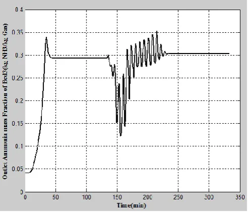
Constant C ensures that u ≥ 0.5. Simulation results are shown in Figure 6.

Fig 6: Disturbed Reactor Outlet Temperature and concentration using PID controller.

When the system is subjected to disturbance due to reducing the feed temperature, the reactor suffers from temperature oscillations. The PID controller tries to overcome the reduction in feed temperature by adjusting the quench valves. The system has temperature oscillations for about 105 minutes. The temperature reaches its min. value at 272.2°C then stabilizes at 500°C. So the temperature drop was about 45.56% from the normal value.

Also , high oscillations in the ammonia outlet concentration, which reach their min. value at 12.19%. Then, after 105 minutes, the system stabilizes with 30.29% ammonia concentrations.

From Figure 6 it is clear that, the system suffers from high oscillation for about 105 minutes, which is along time taken by the controller to overcome the disturbance.

9.

VARIABLE STRUCTURE CONTROL

FOR MULTIVARAIBLE SYSTEM

Consider a multivariable system described by the state equation:

Lx y

Bu Ax x

  



(11) where

x(t) is the state vector, u(t) is the input vector, y(t) is the output vector and A,B,L are constant matrices. The sliding surface is chosen in error domain as:

e C S_ T

(12) where C is a parameter matrix. The error is defined as

x x

e d  ₍₁₃₎

where xd is the desired state. The error derivatives are the state variables

) ( ) ( ...

1 ,.., 1

2 2 1 1

1

t d t u e a e a e a e

n i where e

e

n n n

i i

     

  

  

ueq and a hitting control input uh, it has the following control

law:

h eq u u u 

(15) With Sliding Condition

0 lim ,

0 lim

0

0  

  

s s

s

s ₍₁₆₎

At S(x)



=S(x)= 0 is called a switching surface or switching hyperplane as in Figure 7.

Fig 7: The Sliding surface (S)

The Equivalent control ueq is given by:

) ( ) (

... ) ( )

(

0 ) ( )

( ... ) (

0 ...

0 ) (

1 ...

0

1 2

1 2 1 1

1 2

1 2 1 1

1 1 2

2 1 1

1 1 2

2 1 1

t d e c a e

c a e a t u

t d u e c a e

c a e a

e e c e

c e c

t e C S

c where e

e c e

c e c S

n n n eq

eq n n n

n n n T

n n

n n

 

     

   

   

  

 

 

 

    

 

 

  

  

 

(17)

So the control input u can be expressed as

h n

n

n c e dt u

a e

c a e a t

u() 1 1( 2 1) 2...(  1)  ()

(18)

10.

DECOMPOSITION OF

MULTIVARIABLE SYSTEM INTO

SUBSYSTYEMS

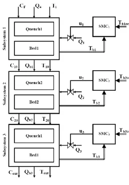
Since it is required to produce a control input u(t) that will be applied to the system. To reduce the complexity of the system, the ammonia reactor system can be decomposed into three subsystems (see Appendix B), each subsystem contains single Quench and single Bed this can be as shown in Figure 8.

Fig 8: Subsystems of Ammonia Reactor

Each subsystem has its own sliding mode controller with the following sliding equations:

1 1 1

1 3

1 2

1 1

 

 

 







  

r r

k k k

m m

j j j

n n

i i i

c and e c S

c and e c S

c and e c S

(19) where

3 3

2 2

1 1

kb ref kb k

jb ref jb j

ib ref ib i

T T e

T T e

T T e

 

 

 

(20)

So SMC Controller uses control low is expressed as

) (S Msat u

u eq ₍₂₁₎

where M is positive constant.

11.

SIMULATION RESULTS

In this section, the validity and effectiveness of the proposed controller scheme are examined through the fast recovery and the stability of the system. Compare these results with traditional PID controller.

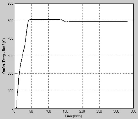
Figure 10 shows a stable behavior of the reactor regardless 50% constrains and the temperature disturbance. When a sudden change in the feeding temperature at time 135mins. There are little ripples in the mass concentration due to the temperature disturbance. The outlet mass concentration is about 31%. But, when applying the disturbance there is some little oscillations for 5 mins. Approximately, then the system stabilized after 26.5 mins.

Table 1 summarizes the results of the controllers

Table 1. Controllers Comparison

System Compare PID DSMC

Oscillations Very high little

Time of Recovery (min) 105 26.5

Ammonia Concentration 30.29% 31%

Ammonia Quantity(Tons/H) 76.33 78.12

The table shows that DSMC has achieved the fast recovery time with little ripples. It takes 26.5 min to overcome the disturbance. While PID controller has the highest ripples with largest time of recovery.

Fig 10: Disturbed Reactor Outlet Temperature and Concentrations using DSMC controller.

12.

CONCLUSION

This paper presents the design of control system for controlling an Ammonia Reactor using the decoupled sliding mode control algorithm. The decoupled technique divides the system into three subsystems each contains a Quench and a Bed which can be separately modeled and controlled. Subject thereactor to temperature disturbance with adding constraints to the quantity of flow gasses to verify the effectiveness of the controller. Comparing the controller with traditional PID controller which achieves high oscillation in outlet ammonia concentration, illustrates the robustness of the suggested controller.

13.

REFERENCES

[1] L. Hung and H. Chung, “Decoupled sliding-mode with fuzzy-neural network controller for nonlinear systems” International Journal of Approximate Reasoning 46 (2007) 74–97.

[2] V.I. Utkin, “Variable structure systems with sliding mode”: A survey, IEEE Transaction on Automatic Control 22 (1977) 212–222.

[3] M. Chan, C. Tao and T. Lee, “Sliding mode controller for linear systems with mismatched time-varying uncertainties”, Journal Franklin Inst. 337 (2) (2000) 105– 115.

[4] M. Falahpoor, M. Ataei and A. Kiyoumarsi, " A chattering-free sliding mode control design for uncertain chaotic systems", Chaos Solitons and Fractals 42 (2009) 1755–1765 .

[5] G. Bartolini , E. Punta and T. Zolezzi, " Simplex sliding mode methods for the chattering reduction control of multi-input nonlinear uncertain systems", Automatica 45 (2009) 1923-1928.

[6] D. Khadija, L. Majda and N. Said, "New Discrete Sliding Mode Control for Nonlinear Multivariable Systems: Multi-Periodic Disturbances Rejection and Stability Analysis ", International Journal of Control Science and Engineering 2(2) (2012) 7-15.

Systems with State Observer", International Journal of Computational Cognition 8( 2) (2010) 9-16.

[8] L. Hsu, R. Costa, and J. Paulo, "Model-Reference Output-Feedback Sliding Mode Controller for A Class of Multivariable Nonlinear Systems", Asian Journal of Control 5 (4) (2003) 543-556.

[9] K. Kim and Y. Park, " Parametric Approaches to Sliding Mode Design for Linear Multivariable System", International Journal of Control, Automation and System 1 (1) (2003) 11-18.

[10] O. Boubaker, J. babary and M. Ksouri, " MIMO Sliding Mode Control of a Distributed Parameter Denitrifying Biofilter", Applied Mathematical Modeling 25 (2001) 671-682.

[11] T. Wua, J. Wangb and Y. Juang ,”Decoupled integral variable structure control for MIMO systems”, Journal of the Franklin Institute 344 (2007) 1006–1020.

[12] F. Yorgancioglu and H. Komurcugil,” Decoupled sliding-mode controller based on time-varying sliding surfaces for fourth-order systems”, Expert Systems with Applications 37 (2010) 6764–6774.

[13] D. Khadija, L. Majda and N. Said, "New Discrete Sliding Mode Control for Nonlinear Multivariable Systems: Multi-Periodic Disturbances Rejection and Stability Analysis ", International Journal of Control Science and Engineering 2(2) (2012) 7-15.

[14] J. Morud and S. Skogestad, " Analysis of Instability in an Industrial Ammonia Reactor", AIChE Journal 44 (4) (1998) 888- 895.

[15] R. Angira, "Simulation and Optimization of an Auto-Thermal Ammonia Synthesis Reactor", International Journal of Chemical Reactor Engineering 9 (A7) (2011), ISSN 1542-6580, The Berkeley Electronic Press.

[16] A. Murase, H. Roberts and A. Converse, “Optimal Thermal Design of an Auto thermal Ammonia Synthesis Reactor”, Industrial & Engineering Chemistry Process Design Development, 9(4) (1970), pp. 503- 513.

[17] C. Singh and D. Saraf, “Simulation of Ammonia Synthesis Reactors”, Industrial & Engineering Chemistry Process Design Development,18(3) (1979), pp. 364-370.

[18] R. Baddour, P. Brian, B. Logeais and J. Eymery, "Steady-state simulation of an ammonia synthesis converter", Chemical Engineering Science, 20 (1965), pp. 281-292.

[19] T. Mohammad .and K. Azam , "The Optimization of an Ammonia Synthesis Reactor Using Genetic Algorithm", International Journal of Chemical Reactor Engineering 6 (A113) (2008), ISSN 1542-6580, The Berkeley Electronic Press.

Appendix A : Data Model

Gas heat capacity, CPg 3500 J/kg, K Catalyst Heat capacity, CPc 1100 J/kg, K Heat of reaction, - ΔHrx 2.7x106 J/kg NH3

Volume, bed 1 6.69 m3

Volume, bed 2 9.63 m3

Volume, bed 3 15.2 m3

Catalyst bulk density, ρcat 2200 Kg/m3

Typical gas density 50 Kg/m3

Quench1 Q1 mass flow 58 Tons/h

Quench2 Q2 mass flow 53 Tons/h

Quench3 mass flow 32 Tons/h

Inlet flow preheater 127 Tons/h Feed mole fraction NH3 0.0417 % Feed mole fraction N2 0.2396 % Feed mole fraction H2 0.7187 % Feed gas temperature, TF 300 °C Typical reactor pressure, P 170 Bar

Appendix B : Subsystems of Ammonia

Reactor Model

Subsystem1: Which contains Quench1 and Bed1

                                                                                                                                                                                                    10 9 8 7 6 5 4 3 2 1 1 1 1 1 1 1 1 1 1 1 1 1 1 1 1 1 1 1 1 10 9 8 7 6 5 4 3 2 1 0 0 0 0 0 0 0 0 0 0 0 0 0 0 0 0 0 0 0 0 0 0 0 0 0 0 0 0 0 0 0 0 0 0 0 0 0 0 0 0 0 0 0 0 0 0 0 0 0 0 0 0 0 0 0 0 0 0 0 0 0 0 0 0 0 0 0 0 0 0 0 0 0 0 0 0 0 0 0 0 0 x x x x x x x x x x x x x x x x x x x x                                                                                                                                                                                                                                                                                         4 3 2 1 30 9 10 1 9 10 1 8 9 1 8 9 1 7 8 1 7 8 1 6 7 1 6 7 1 5 6 1 5 6 1 4 5 1 4 5 1 3 4 1 3 4 1 2 3 1 2 3 1 1 2 1 1 2 1 1 1 1 1 4 1 1 1 1 1 ) ( * 0 0 ) ( * 0 0 0 ) ( * 0 0 ) ( * 0 0 0 ) ( * 0 0 ) ( * 0 0 0 ) ( * 0 0 ) ( * 0 0 0 ) ( * 0 0 ) ( * 0 0 0 ) ( * 0 0 ) ( * 0 0 0 ) ( * 0 0 ) ( * 0 0 0 ) ( * 0 0 ) ( * 0 0 0 ) ( * 0 0 ) ( * 0 0 0 * 0 0 * ) ( * ) 1 ( Q Q Q Q C T T C C mc Cpc Hrx C C mc Cpc Hrx C C mc Cpc Hrx C C mc Cpc Hrx C C mc Cpc Hrx C C mc Cpc Hrx C C mc Cpc Hrx C C mc Cpc Hrx C C mc Cpc Hrx C C mc Cpc Hrx C C mc Cpc Hrx C C mc Cpc Hrx C C mc Cpc Hrx C C mc Cpc Hrx C C mc Cpc Hrx C C mc Cpc Hrx C C mc Cpc Hrx C C mc Cpc Hrx C mc Cpc Hrx C mc Cpc Hrx Q Q mc Cpc Hrx F F     

Subsystem2: Which contains Quench2 and Bed2

                                                                                                                                                                                                                                                                  4 3 2 1 10 10 19 20 2 19 20 2 19 20 2 18 19 2 18 19 2 18 19 2 17 18 2 17 18 2 17 18 2 16 17 2 16 17 2 16 17 2 15 16 2 15 16 2 15 16 2 14 15 2 14 15 2 14 15 2 13 14 2 13 14 2 13 14 2 12 13 2 12 13 2 12 13 2 11 12 2 11 12 2 11 12 2 11 2 11 2 11 2 4 1 2 2 2 2 2 ) ( * 0 ) ( * ) ( * 0 0 0 0 ) ( * 0 ) ( * ) ( * 0 0 0 0 ) ( * 0 ) ( * ) ( * 0 0 0 0 ) ( * 0 ) ( * ) ( * 0 0 0 0 ) ( * 0 ) ( * ) ( * 0 0 0 0 ) ( * 0 ) ( * ) ( * 0 0 0 0 ) ( * 0 ) ( * ) ( * 0 0 0 0 ) ( * 0 ) ( * ) ( * 0 0 0 0 ) ( * 0 ) ( * ) ( * 0 0 0 0 * 0 * * ) ( * ) ( * Q Q Q Q C C T T C C mc Cpc Hrx C C mc Cpc Hrx C C mc Cpc Hrx C C mc Cpc Hrx C C mc Cpc Hrx C C mc Cpc Hrx C C mc Cpc Hrx C C mc Cpc Hrx C C mc Cpc Hrx C C mc Cpc Hrx C C mc Cpc Hrx C C mc Cpc Hrx C C mc Cpc Hrx C C mc Cpc Hrx C C mc Cpc Hrx C C mc Cpc Hrx C C mc Cpc Hrx C C mc Cpc Hrx C C mc Cpc Hrx C C mc Cpc Hrx C C mc Cpc Hrx C C mc Cpc Hrx C C mc Cpc Hrx C C mc Cpc Hrx C C mc Cpc Hrx C C mc Cpc Hrx C C mc Cpc Hrx C mc Cpc Hrx C mc Cpc Hrx C mc Cpc Hrx Q Q mc Cpc Hrx Q mc Cpc Hrx F F  

Subsystem3: Which contains Quench3 and Bed3