Probabilistic Neural Network Assisted Cell Tracking and Classification

(1)

| Page 1155

Probabilistic Neural Network Assisted Cell Tracking and Classification

Shahana.S.

1

_{, Dr.Dinakar Das.C.N.}

2

_,

1

_{M.tech Student, Applied Electronics and Instrumentation, Lourdes Matha College of Science & Technology}

2

_{Associate Professor, Dept. Of ECE, Lourdes Matha College of Science & Technology}

---*---Abstract — Being the fundamental units of life, cells are**

the key actors in many biological processes. Even today, some of the cell tracking problems are dense populations of cells, presence of complex behavior or poor image quality. The existing cell tracking methods are usually very simple and use only a small number of features to allow for manual parameter tweaking or grid search. In this paper, we propose a PNN classifier for robust cell classification. The objective of this paper is to predict and classify by means of analysis of microarray data. We then use neural network to classify the selected features and compare their precision and recall. The proposed PNN classification technique is robust and achieves higher tracking accuracy. Experimental results verifies the ability of PNN in achieving good classification in compared with traditional PNN or Back Propagation Neural Network (BPNN) and KNN.

Index Terms—cell tracking, probabilistic neural

network, Back Propagation Neural Network, KNN

I. Introduction

In recent years, as microscopy imaging technology has been improved and automated, large volumes of microscopy image data are being generated in biomedical fields. Accordingly, how to efficiently analyze and process the data becomes one of the major challenge in this fields since manual analysis is often not feasible any more. This challenge leads to rapidly increasing attention to computer vision base systems for bio image analysis or algorithms are used for image processing that enable automated and quantitative analysis of visual data.

Cell tracking comprehends all techniques to monitoring the behaviour of live cells, particularly cell growth, migration, and differentiation, is of great importance in order to understand the underlying mechanisms of cell physiology and development. For instance, monitoring cell growth and differentiation is critical for extending our knowledge of both normal and aberrant cell behaviour in physiological processes, such as proper organ development, virus replication, and cancer development. Quantitative Analysis of cell migration is also crucial for investigating

several biological phenomena that involve cell migration, such as embryonic development, wound healing process and metastasis.

The automation of these tasks faces several problems, including the poor image quality (low contrast and high noise levels), the varying cell density due to division and cells entering or leaving the particular field of view, and the possibility of cells touching each other without sufficient image contrast. A computer vision-based system that detects cellular events and tracks individual cells in order to realize an automated long-term monitoring of cell behaviour. The system detects cell division and cell death to measure cell growth, tracks cells to quantify cell migration, and locates differentiated cells to capture cell differentiation. This system aims at helping researchers in biological or biomedical sciences to more efficiently determine the effect of exogenous biochemical or physical signals on the activity of cell.

(2)

| Page 1156

II Literature Review

Over the past decade, large number of cell tracking algorithms have been developed. These algorithms concentrate on cell types and are based on different visual tracking methods. In general, they can be divided into two categories, with respect to the tracking paradigm used. The first consists of algorithms based on the “first detect, then track” principle. These algorithms first perform detection of all cells in the whole image sequence and then make links between detected cells from frame to frame based on certain criteria. Examples of such algorithms are include [1], [2]–[4]. The main characteristic of this approach is its computational efficiency with respect to segmentation, but the algorithms often encounter problems during the temporal data association stage [4]. Especially, this is the case for high cell densities tracking data, large numbers of cell division events, and cells entering and leaving the field of view, i.e., when it is difficult to determine the exact number of active cells in the current frame [6]. Every case of splitting or merging some of the tracks established requires a special treatment procedure required for it. Usually, such cases are resolved by using information from the adjacent frame(s). Development of an efficient splitting or merging procedure often requires training on large numbers of features, thus making such approach harder in practice. During the segmentation step is another weakness of this type of algorithms that, usually no information about the segmentation of previous frames is used.

The second category of algorithms uses segmentation and tracking scheme, which, combined with contour models [7]. The idea behind this type of tracking is that for each object a model is created that describes the object being tracked. In this case, segmentation and tracking are performed same time by fitting the model to the image data and using the end result in one frame as the initial step for segmentation in the next frame. One example of this type of tracking is the mean shift process [8], which works well in case of tracking cells of known shape showing relatively small displacements between frames. Another for this model is active contours, which in the last few years became the first choice for model-evolution- based cell tracking [9] In practice, active contours can be implemented explicitly, via a parameterization (e.g., snakes), or implicitly, using the level set framework. Active contours can in principle perform tracking on any cell image sequences, but they can also be tailored to a specific application by putting, e.g., size or shape constraints. The main advantage of the model evolution

based approach is that each object being tracked preserves its identity, and events changing the total number of objects,( cells entering, or leaving the frame) can be handled more easily. The other advantage is that all available information from the previous step can be directly incorporated into the segmentation of the current image frame. This leads to much more accurate results in comparison to algorithms based on separated segmentation and tracking. The main drawback of the model evolution approach is that it is often rather expensive from a computational point of view.

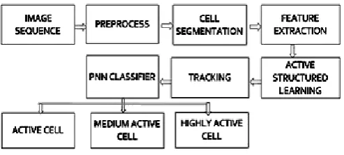
III.Block Diagram

Image sequence:

Large number of image sequences are

used as the input.

Image pre-processing:

Image pre-processing is required

to properlyidentify the cells. The pre-processing steps are:

(a) Noise Removal: Median filtering is used to reduce the existing high noise level in the input frames. The median filter is an effective method that can suppress isolated noise without blurring sharp edges. Specifically, the median filter replaces a pixel by the median of all pixels in the neighbourhood.

(b) Contrast enhancement: This method usually increases the global contrast of many images, especially when the usable data of the image is represented by close contrast values. Through this adjustment, the intensities can be better distributed on the histogram. This allows for areas of lower local contrast to gain a higher contrast. Histogram equalization accomplishes this by effectively spreading out the most frequent intensity values. The method is useful in images with backgrounds and foregrounds that are both bright or both dark.

Cell- Segmentation

. To detect the cells in our image a threshold based segmentation is used. Each pixel xiϵ I is classified as foreground or background with

Xi =

(3)

| Page 1157

morphological operation erosion and dilation. First, an

erosion operator is used to separate tiny false connections between cell areas. Then, a dilatation operation is used to fill holes present. Finally, all areas smaller than a minimum size (cells) are deleted in order to remove small particles and cell debris.

Feature extraction:

Common features such as Centroid

[image:3.595.37.284.260.371.2]

Position, Mean Intensity, Std Intensity, Mean Intensity Edge Area, Size, and Shape. However, more complicated features that are typical in the field of digital image processing.

Fig. 1. Diagram of proposed system.

Active Structured Learning Algorithm

: This algorithm

is used for cell tracking. Active learning is a special case of semi-supervised machine learning in which a learning algorithm is able to interactively query the user (or some other information source) to obtain the desired outputs at new data points. In statistics literature it is sometimes also called optimal experimental design.

• Initialize parameter

• arg max q(x , w)

• Select the best tracking with minimum loss

• Update the new parameter

• Verify the stopping criteria

• Iterate the process until get max q(x , w)

(4)

| Page 1158

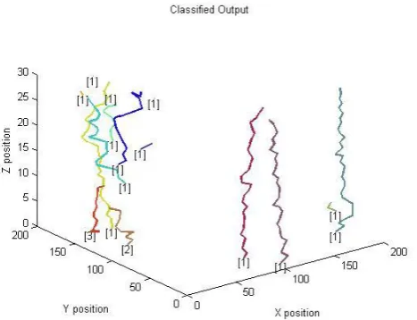
Fig3: Trajectory of lineages

Probabilistic neural networks (PNNs)

Basics

The PNN is based on Bayes–Parzen classification, Bayes theorem for conditional probability and Parzen’s method for estimating probability density function of random variables. The method was not much more use because of the lack of sufficient computation power until recently. The PNN was first introduced by Specht (1990), who showed how the Bayes–Parzen classifier could be broken up into a large number of simple processes and implemented that in a multilayer neural network To understand Bayes’ theorem, consider a sample x=[x1,x2,. . ., xp] taken from a collection of samples belonging to a number of distinct samples (1,2,. . . ., K). Assuming that the hk is the prior probability that a sample belongs to the kth population,

ck is the cost associated with misclassifying that sample, and f1(x), f2(x),. . ., fk(x),. . ., fK(x) aret the true probability density function of all populations are known, Bayes theorem classifies an unknown sample into the ith population if

hici fi(x) > hjcj fj(x) (1)

for all populations j,i. The density function fk(x) examples around the unknown example corresponds to the concentration of class k. From Eq. (1), according to Bayes’ theorem a class that has high density in the vicinity of the unknown sample, or the misclassification cost or prior probability is high. One of the biggest problem in Bayes’ classification approach is the probability density function fk(x) is not usually known. In nearly all standard statistical

classification algorithms, some knowledge regarding the underlying distribution of the samples of all random variables used in classification should be known or reasonably assumed. Most often, Gaussian distribution is assumed; however, the normality assumption cannot always be safely justified. When the distribution is not known and the true distribution deviates considerably from the assumed one, the traditional statistical methods normally run into major classification problems the result is higher misclassification rate. There is a need to derive an estimate of fk(x), from the training set composed of the training example, rather than just assume Gaussian distribution. The multivariate probability density function (PDF)will be the resulting distribution that combines all the explanatory random variables. From a set of training examples to derive such distribution estimator, the Parzen’s method is usually used. The multivariate

PDF estimator, g(x), may be expressed as:

(2)

where 1, 2,. . ., and are the smoothing parameters representing standard deviation (window or kernel width) around the mean of p random variables x1, x2,. . ., xp, W is a weighting function to be selected with specific characteristics , and n is the total number of training examples. If all smoothing parameters are assumed equal (i.e 1, 2,. ), and a bell shaped Gaussian function is used for W.

Network operation

(5)

| Page 1159

first presenting it to all pattern layer neurons. In pattern

layer each neuron computes a distance measure between the presented input vector and the training example represented by that pattern neuron. The PNN then use this distance measure to the Parzen window as weighting function, W and yields the activation of each neuron in the pattern layer. Then the activation from each class is fed to the next corresponding layer of summation layer neuron, which adds all the results in a particular class together. The activation of each summation neuron is executed by applying the remaining part of the Parzen’s estimator equation to obtain the estimated probability density function value of population of a particular class. If the misclassification cost and prior probabilities are equal between the two classes, and the classes are mutually exclusive, that means no case can be classified into more than one class and exhaustive (i.e., the training set covers all classes fairly), the activation of the summation neurons will be equal to the posterior probability of each class. The results from the two summation neurons are then compared and the largest is fed forward to the output neuron to yield the computed class and the probability that this example will belong to that class. The most important parameter that needs to be determined to obtain an optimal PNN is the smoothing parameters of the random variables. A straightforward procedure involves selecting an arbitrary values of ’s, training the network, and testing it on a test set of examples. This procedure is repeated for other ’s and the set of ’s that produces the least misclassification rate is chosen.

Fig:4 A simple probabilistic neural network (PNN) with four input variables, two classes, and eight training examples (five belonging to class 1and three to class 2).

Probabilistic Neural Network Algorithm:

Step 1: Pre-processing of data

 Collect the data for the PNN based prediction algorithm.

 Define the set of values for the training and testing purposes. Here from the literature, the collected. And then transform it to the format of PNN.

Step 2: Training of PNN

 Train the network, with the help of PNN training algorithm, input and output matrices.

 Identify the suitable value of spread constant s. The value of s cannot be selected arbitrarily. A too small s value can result in a solution that does not generalize from the input/ target vectors used in the design. In contrast, if the spread constant is large enough, the radial basis neurons will output large values for all the inputs used to design a network.

Step 3: Testing of PNN

 Define the matrix for the testing of the PNN network.

(6)

| Page 1160

Fig5: cells classified (1).active cell( 2) medium active cell (3)

highly active cell

IV.Classification Accuracy

[image:6.595.48.282.101.280.2]

Decision tree classifier and PNN classifier are compared here. From the data we can clearly understood that the PNN classifier can be more accurately classify the cells.

Fig 6: Comparison of classification accuracy

V. Time Consumption

Fig 7: Comparison of time consumption

Both the original and our proposed methods were implemented in the same experimental programming environment (MATLAB). This allows for a good comparison of computation times. PNN classifier has fast segmentation this will likely reduce the required absolute computation times by a considerable amount, our proposed method will remain substantially faster than the original method.

VI. Conclusion

Developed an automated system capable of simultaneously tracking thousands of individual cells in dense cell populations in phase contrast microscopy image sequences. Here use a new cell tracking scheme that have many expressive features and train the larger number of parameters involved. Further propose probabilistic neural network classifier that, classify tracked cells based on their motion activity.

Reference

[1] X. Lou and F. A. Hamprecht, “Structured learning for cell tracking,” in Neural Inf. Process. Syst., 2011, pp. 1296–1304.

[image:6.595.319.539.124.308.2]

(7)

| Page 1161

[3] F. Yang, M. A. Mackey, F. Ianzini, G. Gallardo, and M.

Sonka, “Cell segmentation, tracking, and mitosis detection using temporal context,” in Medical Image Computing and Computer-Assisted Intervention, J.S. Duncan and Gerig, Eds. Berlin, Germany: Springer-Verlag, 2005, Lecture Notes in Computer Science, pp. 302–309.

[4] D. R. Padfield, J. Rittscher, and B. Roysam, “Spatio-temporal cell segmentation and tracking for automated screening,” in Proc. 2008 IEEEInt. Symp. Biomed. Imag.: From Nano to Macro, Paris, France, 2008, pp. 376–379.

[5] S. Särkkä, A. Vehtari, and J. Lampinen, , P. Svensson and J. Schubert, Eds., “Rao-blackwellized Monte Carlo data association for multiple target tracking,” in Proc. 7th Int. Conf. Inf. Fusion. Mountain View, CA: Int. Soc. Inf. Fusion, Jun. 2004, vol. I, pp. 583–590.

[6] Z. Khan, T. R. Balch, and F. Dellaert, “MCMC-based particle filtering for tracking a variable number of interacting targets,” IEEE Trans. PatternAnal. Mach. Intell., vol. 27, no. 11, pp. 1805–1819, Nov. 2005.

[7] K. Smith, D. Gatica-Perez, and J.-M. Odobez, “Using particles to track varying number of interacting people,” in Proc. IEEE Conf. Comput. Vis. Pattern Recognit., Jun. 2005, vol. 1, pp. 962–969.

[8] Q.Wen, J. Gao, and K. Luby-Phelps, “Multiple interacting subcellular structure tracking by sequential Monte Carlo method,” in Proc. IEEEInt. Conf. Bioinf. Biomed., 2007, pp. 437–442.

Probabilistic Neural Network Assisted Cell Tracking and Classification

| Page 1155