Several Instant Progression Clinical Data Processing For Sorting and Merging With Geometric Measures

© 2016, IRJET | Impact Factor value: 4.45 | ISO 9001:2008 Certified Journal

| Page 241

SEVERAL INSTANT PROGRESSION CLINICAL DATA PROCESSING FOR

SORTING AND MERGING WITH GEOMETRIC MEASURES

*1

_{Ms. Arun kumari G., *}

_{Mrs. Sangeetha Lakshmi G.,}

*1

_{M.Phil Research Scholar, Department of Computer Science, D.K.M. College for Women (Autonomous), Vellore,}

TamilNadu, India.

*2

_{Assistant Professor, Department of Computer Science, D.K.M. College for Women (Autonomous), Vellore,}

TamilNadu, India.

---***---Abstract

causes of death for 31 consecutive years in India. Radiofrequency ablation (RFA) is a treatment for hepatocellular carcinoma (HCC) and it becomes one of the important therapies for HCC these years. For those who had HCC and were treated by RFA, their clinical data are collected to build predictive models which can be used in predicting the recurrence or not of liver cancer after RAF treatment. Clinical data with multiple measurements are merged based on different time periods and these data are further transformed based on temporal abstraction (TA). Data processed by TA reveal variations of clinical data with different time points. The goal of this study is to evaluate whether clinical data handled by TA could facilitate performance of predictive models. Different data sets are used in developing predictive models, including clinical data which are not processed by TA called the original data set, clinical data which are processed by TA called the TA data set, and combination of the original data set and the TA data set called the TA+ original data set. Multiple Measures Support vector machine (MMSVM) was selected as a classifier to develop predictive models. Based on The results demonstrate data sets processed by TA provide benefit for predictive models.

Key Words:

Medical Transcription system, Medical

Care, Temporal abstraction, hepatocellular

carcinoma, Radio frequency ablation, Multi

measures Support vector Machine.

I. INTRODUCTION

The Ministry of Health and Welfare, India, announced the “Causes of Death in India, 2012”. Cancer has ranked first for 31 consecutive years and liver cancer was one of leading causes of cancer death in India [1]. Radiofrequency ablation (RFA) becomes one of important treatments for these years. There are many advantages of RFA. For example, it can destroy the cancer cells clearly, be operated repeatedly, and patients can take less risk of anesthesia than traditional therapy. Literature shows that small scale hepatocellular carcinoma received RFA as the initial treatment, 1-year survival rates is 96% and more than 50% in 5 years [2]. Early detection of liver cancer is not easy, and patients not treated timely or actively are the reason for high mortality. In this research, we use the cohort information from HCC patients to build predictive models for predicting patients’ HCC recurrences after RFA in one year. There are useful technologies for analyzing the existing data, such as data warehousing, data mining and data prediction. We should determine the data type before data processing. Data could be divided into two types, cross-sectional data and time series data.

© 2016, IRJET ISO 9001:2008 Certified Journal

Page 242

transformation may improve the performance and efficiency of mining by transforming original data. Transforming data from a low level quantitative form to high-level qualitative description is known as temporal abstraction (TA). The process of TA takes either raw or pre-processed data as input and produces context sensitive and qualitative interval based representations. In this study, original data sets are regarded as input and trends of features (increase, decrease, and unchanged) are produced by TA.

In this study, different data sets are used in developing predictive models, including clinical data which are not processed by TA called the original data set, clinical data which are processed by TA called the TA data set, and combination of the original data set and the TA data set called the TA+ original data set. Performance of three types of models built based on different data sets are compared. Multi Measures Support vector machine (MMMMSVM) was selected as a classifier to develop predictive models.

1.1This paper makes the following contributions:

 We propose a method using MTGP for forecasting patient acuity based on irregularly sampled heterogeneous clinical data.

 We propose a new latent space for representing multidimensional time series using inferred MTGP hyper parameters.

 We evaluate our approach in two ways: 1) estimating and forecasting a cerebrovascular auto regulation index from noisy physiological time-series data in patients who suffered a traumatic brain injury and 2) transforming irregular ICU patient clinical notes into time series, and using MMMMSVM hyper parameters from these time series as features to predict mortality probability.

II. METHODS

2.1. DATA SOURCE

We use the data from the HCC patients who have received RFA as the initial treatments for HCC from 2012 to 2013 in NTUH (National India University Hospital for developing and evaluating a proposed approach in this study.

In this study, total 26 clinical features are included. There are 20 laboratory items, including prothrombin time international normalized ratio (INR), albumin, aspartate aminotransferase (AST), alanine transaminase (ALT), alkaline phosphatase, total bilirubin, hepatitis C virus (HCV), hepatitis B virus (HBV), alpha-fetoprotein, sodium (Na), potassium (K), creatinine, blood urea nitrogen (BUN), hemoglobin, hematocrit, white blood cell count, platelet

count, direct bilirubin-GT, and total protein. There are two demographic data items, including gender and age.

There are four features extracted from medical textual reports, including Barcelona clinic liver cancer (BCLC) staging classifications, liver cirrhosis, the size of the maximal tumor, and the number of tumors. medical students on their orthopedics rotation, preparing to observe their first arthroscopic knee surgery, will be able to go the school's electronic learning center and use the Internet to access and manipulate a three-dimensional "virtual reality" model of the knee on a computer at the National Institutes of Health. They will use new immersive technologies to "enter" the model knee, to look from side to side to view and learn the anatomic structures and their spatial relationships, and to manipulate the model with a simulated arthroscopic, thus getting a surgeon's-eye view of the procedure before experiencing the real thing.

2.2 The Algorithm for Merging Multiple Features

Based on Time Period

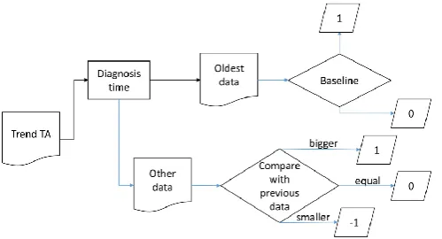
The algorithm for merging multiple features (i.e., 20 laboratory items) based on time period is presented in Figure 1. Figure 1 shows an example for merging multiple features every 30 days. In this study, different periods are tested, including 7, 14, 21, 30, 60, 90, and 120 days.

There might be more than one value of a feature in each period and only the value closest to treatment date would be taken.

Figure1. An example for Time Period in 30 days

2.3. Temporal abstraction

© 2016, IRJET ISO 9001:2008 Certified Journal

Page 243

to present their trend (increase, decrease, and unchanged), except HBV and HCV (Figure 3).

Figure 2. The flowchart of the temporal abstraction for trend features

Figure 3. An example for Temporal abstraction

2.4. Classification Methods

In the following, MMSVM is introduced. MMSVM uses a nonlinear mapping to transform the original training data into a higher dimension. Within this new dimension, it searches for the linear optimal separating hyper plane [8]. With an appropriate nonlinear mapping to a sufficiently high dimension, data from two classes is guaranteed to be separated by a hyper plane. The MMSVM finds this hyper plane using support vectors and margins (defined by the support vectors) [9]. The advantages of MMSVM include highly accurate, having the ability to model complex nonlinear decision boundaries, and less prone to ove fitting. In addition, a comparison of the MMSVM to other classifiers has been conducted by Meyer [10]. The MMSVM indicates mostly significant performances both on classifications and regression tasks. In this research, the MMSVM library was used for implementing the MMSVM classification method. The LIBMMSVM library provides a complete classification process based on MMSVM, including scaling, training, prediction, grid search, and cross validation function. 5-fold cross-validation is used in this study and random forest is

used for selecting features from a data set. Features are sorted by their importance and added in MMSVM one by one for training to build a predict model.

2.5 Performance evaluation

The performance of classification using the original data was compared with using the processed data by TA by the following performance metrics.

True positive (TP): A positive event correctly identified as a positive event.

False positive (FP): A negative event wrongly identified as a positive event.

True negative (TN): A negative event correctly identified as a negative event.

False negative (FN): A positive event wrongly identified as a negative event.

III. PREVIOUS IMPLEMENTATION

In the clinical world, there are practical examples of data being used to infer patient acuity in the form of ICU scoring systems. ICU scoring systems such as SAPS (simplified acute physiology score) use physiologic and other clinical data for acuity assessment. However, in 2012 scoring systems were used in only 10% to 15% of US ICUs (Below and Badawi 2012). Recent work has focused on feature engineering for mortality prediction. This is usually accomplished by windowing or aggregating the structured numerical data so that a single feature matrix can be fed into a structured deterministic classifier.

Time series Abstraction

© 2016, IRJET ISO 9001:2008 Certified Journal

Page 244

signals into higher level representations. For example, Fox et al. used beta processes to model multiple related time series (Fox et al. 2011), and Marlin et al. used Gaussian mixture models on the first 24 hours of monitor-signals data with hourly-discretization (Marlin et al. 2012). Nevertheless, latent variable approaches are unable to cope with missing and unevenly-sampled data as is, and require either strong assumptions about observations when they change asynchronously, or the computationally expensive approach of modeling time between observations directly as another latent variable.

3.1 Multi-Task Gaussian Process Models

The general STGP framework may be extended to the problem of modeling m tasks simultaneously where each model uses the same index set x (e.g., physiological or clinical time series). A native approach is to train a STGP model independently for each task, as illustrated in Figure 2. We introduce instead an extension to multi-task GP models proposed in (Bonilla, Chai, and Williams 2007), which makes use of the covariance in related tasks to reduce uncertainty in the inferred signal. Let Xn = fxj i j j = 1; :::; m; i = 1; :::; njg and Yn = fyj i j j = 1; :::; m; i = 1; :::; nj ; g be the training indices and observations for the m tasks, where task j has nj number of training data. We consider the regression model ~yn = g(~xn_{) + _, in which g(x) represents the latent function and _ _} N(0; _2n _{) is a noise term. GP models assume that the} function g(~xn) can be interpreted as a probability distribution over functions such that ~yn = g(~xn_{) GP} m(~xn_{); k(~x}n_{; ~x}0 _{n), where(~xn) is the mean function of} the process (assumed = 0) and k(~xn_{; ~x}0 _{n) is a covariance} function describing the coupling among the independent variables ~xn _{as a function of their kernel distance. To} specify the affiliation of index xj i and observation yj i to task j, a label lj = j is added as an additional input to the model,

Fig4: Intracranial Pressures

An example of a single-task GP (STGP) and multi-task GP (MTGP) applied to intracranial pressure (ICP) and mean arterial blood pressure (ABP) signals from a traumatic brain injury patient. (a) and (c) show the performance of STGP, whereas (b) and (d) show the improved performance of MTGP, which takes into account the correlation between ICP and ABP. Dots represent observations, crosses represent missing observations (test observations), the dotted line shows the function mean and the shaded area show the 95% confidence interval. We note that the timescale parameter “selected” by the MTGP, which takes into account the correlation between the tasks, is shorter than the one selected by the STGP, which yields to higher likelihood of the test observations (crosses).

3.2 Hyper parameter Construction

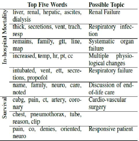
Once notes were transformed into multi-dimensional numeric vectors, we used the MTGPs to model the per-note change in topic membership over a patient’s stay. This is critical for comparing two patients’ records given that patients have different lengths of stay and note taking intervals depend on staff, clinical condition, and other factors. From the topic enrichment measure, we chose the topics with a posterior likelihood above or below 5% of the population baseline likelihood across topics. This yielded nine for a summary of the chosen topics, and the Appendix for more details).We employed MTGP to learn the temporal correlation between the nine topics and the overall temporal variability of the multiple time series.

© 2016, IRJET ISO 9001:2008 Certified Journal

Page 245

features that will discriminate between different classes is of key importance in modeling. A combination of approaches, including literature review, concept mapping, and statistical analysis are several methods that can be used to identify plausible features. Ideally, features should describe the target, correlate with the target, or have other plausible associations with the target.

Table 1: Comparison hyper Parameter Construction

IV. SYSTEM IMPLEMENTATION

4.1 Partition Data Sets

Once the data have been normalized, they are ready for modeling. Although the entire data set could be used to train a model, the ability of that model to perform in unseen data (its external validity) would be undetermined. Models should not be put into use until their external validity has been determined. There are two ways to establish external validity. The gold standard is to employ the model in a prospective fashion and measure its prediction accuracy over time, noting any degradation that may occur as a result of changing practices or disease prevalence. However, this is a laborious process and typically is not undertaken unless some measure of how well it is likely to perform already exists.

Therefore, in order to estimate the external validity, a random portion of samples usually is withheld so that they are never accessed during the training process. Determining how many samples to withhold involves a tradeoff:

withholding too many samples may degrade the model’s performance, whereas withholding too few samples may inaccurately estimate the model’s external validity. Depending on how many examples are in the data, between 20 and 50 percent of the samples typically are withheld for validation as the final step in assessing model performance

4.2 Create Modeling Data Subsets

The final step in preparing to generate predictive models from time series data is to determine what actually belongs in the model. The effort that was put into selecting candidate features, specifying their properties and format, and deriving additional clinically relevant and trend features has provided a comprehensive set of candidate features that are suitable for modeling, but all may not be necessary or appropriate for modeling. From this comprehensive set of features, any number of data subsets can be instantiated to answer the question of “Did that step help improve the model?” In order to answer the question, two or more subsets of the comprehensive data set need to be evaluated through a formal modeling process that involves training and tuning on one data set, and measuring their performance in another. Relative performance from one reference set to the other serves as a measure of the utility of the candidate features that differ between them.

4.3 Reduce Candidate Features

Many modeling algorithms are able to discriminate even the subtlest differences between case and control classes of data. When the number of examples is small and the number of variables that the model can use is large, modeling algorithms are prone to memorize the classes. If this occurs, the preliminary results of the model accuracy will be superb, but the model will fail to predict classes accurately in the validation data set. In order to prevent this problem, feature reduction is frequently employed prior to training to reduce the number of candidate variables to a number less than the algorithms need to achieve memorization.

© 2016, IRJET ISO 9001:2008 Certified Journal

Page 246

Fig5: Time Series Division

4.4 Outcome Classification

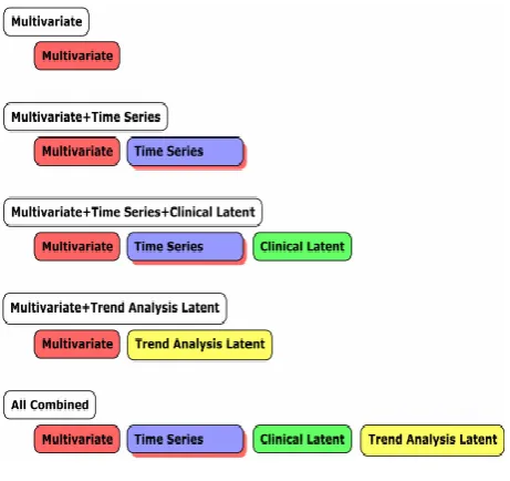
We considered five feature prediction regimes that combined subsets of the feature matrices 1, 2, and 3 as an aggregate feature matrix. We trained two supervised classifiers that were identical in the five feature sets used, but provided different objective functions for optimization: Lasso logistic regression and L2 linear kernel MMSVM. Classifiers were trained to create classification boundaries for two clinical outcomes: in-hospital mortality and 1-year post-discharge mortality. All outcomes had large class imbalance (e.g., in-hospital mortality rates of 10.9%). To address this issue, we randomly sub-sampled the negative class in the training set to produce a minimum 70%/30% ratio between the negative and positive classes. Test set distributions were not modified, and reported performance reflects those distributions. Due to space constraints, we only reported results on a completely held out test set. We performed 5-fold cross-validation on the remaining data, and cross-validation results were similar to those obtained on the completely held-out test set. We evaluated the performance of all classifiers using the area under the Receiver Operating Characteristic curve (AUC) on the held-out test set. Table 3 reports results from the Lasso model. Results obtained using the L2 linear kernel MMSVM was not statistically different.

Table 2: Comparison of Detection Methods

Fig 6: Electronic Medical Record

We selected two strategies that had proven performance in microarray analysis: recursive feature elimination (RFE), which removes features independent of the modeling algorithm, and support vector machine weighting (MMSVMW), which adds features based on weights assigned during SVM model training. Given that both of these techniques are sensitive to interdependencies among variables for a given

outcome (i.e., they will retain two or more variables that work together to make a prediction, even if neither in isolation is highly correlated with the outcome), and that the modeling tool we were using (MATLAB Spider) supported these techniques, we chose them over the simpler, correlation-based techniques. In order to estimate the degree of over-fitting, if any, we also trained candidate modeling data sets without employing feature reduction and compared their performance to those that were trained with feature reduction

V. RESULT AND DISCUSSION

© 2016, IRJET ISO 9001:2008 Certified Journal

Page 247

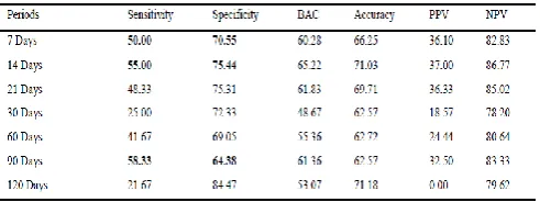
Table 3: The performance of predictive models based on the original values of 26 features

Table 3 and Table 4 show the performance of predictive models based on the TA data sets. In Table 3, the oldest value (the baseline of TA) is set as “0” and in Table 4 the oldest value (the baseline of TA) is set as “1”.

Table 4. The performance of predictive models based on the TA values, totally 26 features, baseline is 0

Table 5. The performance of predictive models based on the TA values, totally 26 features, baseline is 1

Table 4 and Table 5 show the performance of predictive models based on the TA+ original data sets. It has 18 features that are processed by TA, so this dataset totally has 26+18 features. In Table 4, the oldest value (the baseline of TA) is set as “0” and in Table 5 the oldest value (the baseline of TA) is set as “1”.

Table 6. The performance of predictive models based on the TA+ original values, totally 44 features, baseline is 0

Table 7. The performance of predictive models based on the TA+ original values, totally 44 features, baseline is 1

5.1 Discussion

Comparing results of Table 2 with those of Table 2 and Table 3, the values treated with TA or not, if we set the oldest value as baseline is 0 (Table 3), all sets of sensitivity and specificity are less than 50, even less than the original values (Table 2). In Table 4 (set baseline as 1), 3 sets of sensitivity and specificity are not less than 50, there are “7”, “14”, and “90 days”, 2 more than the original data. Comparing results of Table 1 with those of Table 5 and Table 6, the information adds the value treated with TA or not, if we set the oldest value as baseline is 0 (Table 4), “14”, “21”, “30”, and “60 days”, 4 sets of sensitivity and specificity are not less than 50, especially “21” and “60 days” are not less than 60. Set baseline as 1 (Table 6), in all

days, sensitivity and specificity are not less than 50, but only “60 days” better than 60. The results about the baseline value (0 or 1) can be compared between results of Table 3 and Table 4, Table 4 and Table 5. There are 18 features treated with TA, in the results of Table 3 and Table 4, the original values are modified as TA values and no other information are added in these data when baseline value is set as 1 (Table 4), both sensitivity and specificity in “7”, “14”, “90 days” are not less than 50 which are better than the results of Table 3. When data are treated by TA, baseline with 1 provides better results. In Table 5 and Table 6, both original data and TA data are included in data sets. When the baseline is set as 0 (Table 4), in the sets of ”14”, “21”, ”30”, and “60 days”, both sensitivity and specificity are not less than 50. When the baseline is set as 1 (Table 6), in all sets, both sensitivity and specificity are not less than 50. Similarity, baseline with 1 provides better results.

© 2016, IRJET ISO 9001:2008 Certified Journal

Page 248

these are limitations for our study here. Given that the hyper parameters were optimized from pernote topic features (that are themselves the output of an unstructured learning problem), it is most sensible that the topics information should be used in combination with the MTGP hyper parameters to describe patient state. We obtained improved predictive performance for both mortality outcomes when combining both MTGP hyper parameters with SAPS-I and the significant topics. This is likely because the hyper parameters provide complementary information to both SAPS-I and the significant topics.

VI. CONCLUSION

After comparing these results, the data sets treated by TA are more meaningful than data sets not treated by TA. Furthermore, when we add the original data values to the data sets which have been treated by TA, the results will become better than those only with TA values. According to these results, when we treat data by TA, the value of baseline could also influence the performance of predictive models and baseline set as 1 is better than baseline set as 0.The Future values of performance measures do not make the significant impact. For the on-going research, we may add more TA conditions about their relationships between values. Furthermore, we will reduce the number of features and only extract the features with high contribution to performance.

REFERENCES

[1] E. Y. Ministry of Health and Welfare, India, "Causes of death in India, 2012," M. o. H. a. W. Department of Statistics, Ed., ed: Department of Statistics, Ministry of Health and Welfare, 2013.

[2] S. Shiina, R. Tateishi, T. Arano, K. Uchino, K. Enooku, H. Nakagawa, et al., "Radiofrequency ablation for hepatocellular carcinoma: 10-year outcome and prognostic factors," The American journal of gastroenterology, vol. 107, pp. 569-577, 2012.

[3] J. Han and M. Kamber, Data mining: concepts and techniques, 2 ed. San Francisco: Morgan Kaufmann, 2006.

[4] M. Lenzerini, "Data integration: a theoretical perspective," presented at the Proceedings of the twenty-first ACM SIGMOD-SIGACT-SIGART symposium on Principles of database systems, Madison, Wisconsin, 2002.

[5] A. A. Hancock, E. N. Bush, D. Stanisic, J. J. Kyncl, and C. T. Lin, "Data normalization before statistical analysis: keeping the horse before the cart," Trends in Pharmacological Sciences, vol. 9, pp. 29-32, 1988.

[6] Y. Shahar, "A framework for knowledge-based temporal abstraction," Artificial intelligence, vol. 90, pp. 79-133, 1997.

[7] M. Stacey and C. McGregor, "Temporal abstraction in intelligent clinical data analysis: A survey," Artificial Intelligence in Medicine, vol. 39, pp. 1-24, 2007.

[8] C. Cortes and V. Vapnik, "Support-Vector Networks," Machine learning, vol. 20, pp. 273-297, 1995.

[9] B. E. Boser, I. M. Guyon, and V. N. Vapnik, "A training algorithm for optimal margin classifiers," presented at the Proceedings of the fifth annual workshop on Computational learning theory, Pittsburgh, Pennsylvania, United States, 1992.

[10] D. Meyer, F. Leisch, and K. Hornik, "The support vector machine under test," Neurocomputing, vol. 55, pp. 169-186, 2003.

BIOGRAPHIES

1.

Ms.Arun Kumari G, M.Sc,

M.Phil,

Research Scholar, department of

computer science, D.K.M. College for

Women

(Autonomous),

Vellore,

TamilNadu .

2. Mrs. Sangeetha Lakshmi G., Asst.

Prof

Department of Computer Science,