Improved Modeling of System Response in List Mode EM Reconstruction of Compton
Scatter Camera Images
Scott
J.
Wilderman,
J.A.
Fessler, N.H. Clinthorne, and W. Les Rogers
University of MichiganAbstract
An improved List Mode EM method for reconstructing Compton scattering camera images has been developed. First, an approximate method for computation of the spatial variation in the detector sensitivity has been derived and validated by Monte Carlo computation. A technique for estimating the relative weight of system matrix coefficients for each gamma in the list has also been employed, as has a method for determining the relative probabilities of emission having some from pixels tallied in each list-mode back-projection. Finally, a technique has been developed for modeling the effects of Doppler broadening and finite detector energy resolution on the relative weights for pixels neighbor to those intersected by the back-projection, based on values for the FWHM of the spread in the cone angle computed by Monte Carlo. Memory issues typically associated with list mode reconstruction are circumvented by storing only a list of the pixels intersected by the back-projections, and computing the weights of the neighboring pixels at each iteration step. Simulated projection data has been generated for a representative Compton camera system (CSPRINT) for several source distributions and reconstructions performed. Reconstructions have also been performed for experimental data for distributed sources.
I .
INTRODUCTION
List mode Expectation Maximization (EM) methods [ I , 2, 31 are appealing in the Compton camera reconstruction problem because the total number of detected photons is significantly smaller than the number of possible combinations of position and energy measurements, leading to a much smaller problem than that faced by traditional iterative reconstruction approaches. For a realistic device, the number of possible detector bins can be as large as 10 billion per pixel of the image space, whereas the number of counted photons would typically be a fraction of a percent of that. Though memory and computation speed are still important issues (10
million particles in a 128 x 128 images space requires that 1010 weights be stored and computations made at each step), the primary difficulty in applying the list mode technique is in modeling system response for performing the successive back and forward projection operations.
The conventional (binned, data) ML problem for the Compton camera can be posed as follows: Let Y be the measured projection data, accumulated in bins as the number of counts for a given combination of scatter detector element,
'This work has been partially supported through Contract NCI
2RA01 CA-32846-24.
capture detector element, and scattering energy bin (with the number of counts in each bin denoted Yi), and the underlying pixelated object, each pixel having an intensity given by X j . The iteration, (indexed by I ) , is given by
where, s j is the sensitivity, or the probability that a photon emitted from pixel j would be detected anywhere, and t i j the probability that a 7 emitted from pixel j is collected in bin i , so
In the list mode case, we approximate Y by considering that each event is measured in a unique bin, so that Y; + 1 for each detected particle, and Yi + 0 for the infinite number of possible events not detected in the given measurement. The sums over
the
M S
system bins in the above equations become insteadsums over just the N , detected events. Barrett et a1[2] and Parra [3] have proven that this approximation on Y holds (here we ignore any time dependence of the measurement), with the one exception that as the detected Y, no longer span the space of all possible events, s j
#
Ci
tij, but rather, s j is now the integral over all possible events i , including those for which= 0.
In an earlier work [ 5 ] , a simple method for determining the required system matrix coefficients needed in the EM algorithm was developed, by assuming uniform sensitivity and perfect energy and spatial resolution in the detectors. Doppler broadening of the Compton scattered photon energy spectrum was also ignored. These approximations limited the possible emission positions for a given detected event i (in 2D) to those points along conic sections traversing the image plane. The probabilities t i j were then approximated as some constant times the line integral of the conic through pixel j . This technique had two main advantages, in that because of the uniform sensitivity approximation, the method is independent of the system, and in that the coefficients tij could be generated trivially during an initial back-projection operation [7] done to obtain a starting image. Further, it was found that for an N by N image, typically 2N pixels would lie on a conic section, saving a factor of N / 2 matrix element computations.
In the current work, we introduce a simple method for approximating the sensitivities for any Compton device with a planar first detector, and approximations for modeling more than N / 2 pixels per gamma at no increase in storage cost.
11. METHODS
Straight-forward computation of the sensitivities s, and matrix elements tij would require for each gamma in the list a integrations over the areas of each pixel, the entire first detector ands the entire second detector, probabilities and density functions describing the interaction and measurement of the two interaction positions and the scattering energy. As
this is computationally intensive and requires detailed a priori knowledge of all system components, we seek alternative approaches, as described below.
First, the relative spatial variation in the sensitivities sj is assumed to be dominated by just two effects, the solid angle subtended by the scatter detector and the probability of interaction inside the detector. This is justified by noting that after the first Compton scatter, the main efficiency effects (absorption of the scattered photons in the scatter detector and the solid angle subtended by the capture detectors) depend only on the exit angle and hence only on the scattering angles. For systems with large first and second detector areas, most gammas will scattering into angles subtended by the second detector, angle, and so the sensitivity effects after the first scatter will be fairly uniform across the image space. We thus approximate the relative sensitivity for pixel j as the sum of the probabilities of the two first detector geometrical effects taken over all the
D1
first detector elements, leading to(3)
where the ut is the total cross section in the scatter detector, zjl is the pathlength inside the first detector element along the ray from the center of pixel j to the center of each detector element rn and djl the distance between the centers.
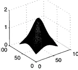
An image map of the relative sensitivities determined for a typical detector configuration using this approach is shown in figure 1, for a 64 by 64 image space covering 30 cm. The method
. . .
1c
Fig. 1 Approximated relative sensitivities
was validated by comparing results to those generate by a Monte Carlo computation. The detector modeled was the prototype C- SPRINT device, consisting of a 32 by 8 array of 1.4 mm silicon detector elements 1 mm thick for the first detector [4] and the SPRINT second detector.
Center Half-Edge
Edge 0.33
0.52
[image:2.612.326.511.98.206.2]Comer 0.17
Table 1
Comparison of Monte Carlo and approximate computation of sensitivities
Agreement is very good, especially considering that the C- SPRINT geometry, with the short second detector (11 cm) and the first detector recessed inside the SPRINT ring is very likely to accentuate any spatially varying effects caused by incomplete solid angle coverage of the second detector and re-absorptions in the first detector because of non-uniform average escape track lengths inside the first detector.
As noted above, straight-forward computation of the weights would require the computation of integrals over 3 position and 1 energy variables for each gamma, a total of N 2 N-, results. We use here an approach requiring computation of just N-, back-projections and just 2NN7 stored results. The approximation of tij is done in a three part fashion. We begin with the original model in which the weights are computed for only those pixels which are intersected by the back-projected cone of each measurement i. As we seek to compute the relative values of the weights (from 1 we note that the iteration is independent of any normalization on the t i j ) , we note that we require 2 factors. The first describes the relative probabilities between the measurements i; the second describes the the probabilities within the measurements, i. e., the probability that the gamma giving rise to the measurement i was emitted from pixel j.
We assume that the first factor is determined primarily from the relative differential cross section and the escape probability of the scattered photon in the first detector:
(4)
where ut is the total cross section at the scattered photon energy in the first detector, 2 1 2 the distance traveled through the first detector along the ray between the first and second collisions, and
%
the differential Compton cross section. Since we need only to determine functional dependence and not absolute values, we approximate as the Klein-Nishina cross section at the given energy divided by the square of the distance between the 2 collisions.The second factor, the relative probability of a given even having come from a gamma emitted from a given pixel, must take into account the pixel sensitivities sj as well as the resolution loss brought on by Doppler broadening and the finite resolution in the energy measurement. We use our relative sj 's for the first factor here, and then assume that the other effects are described by the angular resolution of back-projected cones determined for a given system [7,4]. We assume that the value of the full width at half maximum of the cone-spread function
dUC
f(i)
0; e x P ( - c T , z l z ) ~ [image:2.612.117.251.505.625.2]is constant for all energies (this is valid for the majority of the energy spectrum in which Compton cameras are designed to function [4]), and that the distribution, which is not Gaussian because of the long Doppler tails, can be modeled by adding to .9 times a Gaussian about the computed standard deviation to 10% of a Gaussian distribution with 3 times the cone spread standard deviation,
where T is the normal distance from the back-projected cone.
The relative value assigned to each pixel would be the integral of this function over the area of the pixel. As we plan to store for each gamma only a list of intersected pixels and to generate the pixel weights of all neighboring pixels at each iteration step, we need to approximate the integrals. If we approximate the conics in the integrals to be linear and have r
<<
U , which corresponds to pixel sizes L less than the cone spread in the image plane, it can be shown that integrals over pixels which are intersected by conics vary in the range from 2-
L 2 / 8 u 2 to 2 - 3L2/4u2 depending upon the orientation of the conics. This can be taken to be constant in most applications, and we therefore have that the relative weight of each pixel j in the computation of t i j for a giveni
is dependent solely on the distance between the pixel of intersection to the neighbor pixel j. Neighbors are determined by taking them along either rows or columns of the image space (depending if the conic intersected the image space in a more vertical or horizontal fashion respectively), so the distance to the rnth neighbor is mL, and the relative weight of that pixel is taken asf(m) 0: .9 exp(-(m~)’/2u’)
+
.I e x p ( - ( r n ~ ) ~ / 2 ( 3 u ) ~ ) .(6)
Since the selection of which neighboring pixels to include is made normal to the conic, even though the integral over the spread function in the pixels is independent of the orientation of the conic, for conics which intersect the image space with slopes not near to 0 or infinity, the distances to the center of the neighbor pixels are smaller than L , and the relative weight for the mth neighbor taken from 6 needs to be adjusted. We do this by multiplying f ( m ) by a relative correction which is equal to 1 for slopes of 1 (which correspond to minimum distances between intersected pixel centers and neighbor centers, and increases
to
where s is the approximate average slope of the conic through the image space (or inverse slope if the intersection is more horizontal than vertical The obvious weakness of the method will be for particles with very small scattering angles, leading to back-projections with large second derivatives, and hence large variations in the first derivatives of the conics in the image space.
To summarize then, the t i j are computed by first determining a list of pixels intersected by the back-projected conic for each gamma, as described in [7]. Next, the relative probability between the measurements f ( i ) is computed
according to 4. At each step of the iteration, the weights are approximated by branching out either vertically or horizontally from the intersected pixels and multiplying f ( i ) first by the sensitivity sj, then by the pre-computed spread function f(rn), and finally by the slope dependent correction f(s) for each of the rn neighbors in both the plus and minus direction. Thus we save EL factor of N / 2 in storage at the expense of 3 extra multiplications per iteration step.
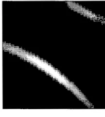
Figures 2 and 3 show the back-projection for a single particle
(i. e., the weights) computed by a lengthy and fairly rigorous method [ 121 and the current approximation. Agreement is seen to be quite.
Fig. 2 Computed back-projections of representative particles
Fig. 3 Approximate back-projections of representative particles
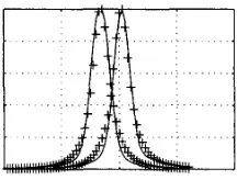
Figure 4 shows
cross
sectional cuts through the image plane of the weights for each method for two sets of back projections, the first with slope very nearly normal to the image space, and the second at close to 45 degrees. The rigorous and approximate models agree well for both cases.111.
RESULTS
ANDDISCUSSION
Results are given below for reconstructions using the current method for both simulated and experimental data. Simulated data was generated using a typical detector configuration and for experimental data using a prototype detector. The system modeled is the C-SPRINT silicon and NaI system proposed by Clinthome and LeBlanc [4]. It consists of a 9x9 cm array of Si
[image:3.616.379.487.403.523.2]Fig. 4 Computed cross sectional back-projections of representative particles
elements, divided into 1.2 mm cells. Each cell is 5 mm thick and assumed to have an energy resolution of roughly 250 eV, (an achievable level, as suggested by Weilhammer [ll]). The capture detector is taken to be a hollow cylinder of NaI, 25 cm in radius and 25 cm long, with a spatial resolution of 3 mm. Projection data was generated by Monte Carlo simulation using the program SKEPTIC [ 6 ] . SKEPTIC has been employed and tested extensively in simulation of Compton scatter cameras
[4, 7, 51. Lists of the exact interaction positions and energy losses are created, and the uncertainties in the measurements of these quantities are simulated by sampling from appropriate Gaussian distributions describing the energy and spatial resolution of the component detectors, as described in [SI. Doppler broadening of the scattered gamma spectrum, which has recently been found to be a limiting factor in the resolution performance of Compton cameras [8], is modeled using the tabulated data of Biggs [9] for amorphous silicon and of Reed [ 101 for crystalline silicon. Simulated spatial configurations of the sources included small Gaussian sources in a warm background, and hot and cold uniform disks of various radii in uniform warm background.
The first image below was generated for a disk source of radius 5 cm with uniform background and 2 cold spots (intensity 0) and 2 hot spots (intensity 2) with 1.0 and .5 cm radii, at a distance of 10 cm from the face of the scatter detector. The reconstruction was done using the current method on a 64
by 64 grid of 3 mm pixels, and modeled the ccne spread by treating 6 pixels on either side of each conic. Both of the hot spots and the cold spots are visible.
Results are shown next for a Gaussian source reconstruction for g g m T ~ . A 64x64 image space of 15 cm FOV was used, and 202,000 detected events modeled. The source consisted of a uniform background disk of radius 7.5 cm, overlayed with a Gaussian of full width at half maximum of 1 cm and maximum intensity 1.4, 10 cm from the front of the silicon detector. Six pixels on either side of the back-projected conics were treated, and a FWHM of 8 mm ([4] was assumed. The initial back-projection and computation of the weights took approximately 3 minutes on a Sparc Ultra workstation and each iteration roughly 40 seconds. Images are shown after iterations
20 and 40.
The final set of images were generated from experimental data taken with the prototype C-SPRINT detector. The phantom in this case was formed by placing a Tcggm line source 7.5 cm long in the shape of a Z. The separation distance between the
[image:4.612.138.246.100.182.2]Fig. 5 Phantom image including Doppler broadening and detector resolution, 50th iteration
Fig. 6 Lesion image after 20th iteration
parallel sections was 7 cm, and the intensity of the angled line
1/2 that of the parallel lines. The FWHM of the cone spread at the 11 cm source to detector distance was computed to be 1.5
cm, and results are shown here for reconstructions after 100 iterations using 0, 8, and 16 pixels on either side of the initial back-projected cones. For the first case, as the 100th iteration image is extremely noisy, only the 20th iteration is shown. Note that there is no discernable improvement in the images quality from treated the tails of the cone spread.
IV.
CONCLUSIONS
A computationally efficient method has been devised for determining the relative sensitivities and system matrix coefficients for Compton scatter cameras with planar first detectors. The method has been shown to give results with excellent agreement in comparison to both Monte Carlo and rigorous analytical results. Images reconstructed from both simulated and experimental data have been presented.
[image:4.612.376.481.103.222.2] [image:4.612.375.482.293.408.2]Fig. 7 Lesion image after 40th iteration Fig. 9 Reconstructed line phantom using 8 nearest pixels, 100th iteration
Fig. 8 Reconstructed line phantom using only central pixel, 20th Fig. 10 Reconstructed line phantom using 16 nearest pixels, 100th
iteration iteration
V.
REFERENCES
[l] T. Hebert, R. Leahy, M. Singh, “Three-dimensional maximum- likelihood reconstruction for an electronically collimated single- photon-emission imaging system,” J. Opt. Soc. Am., vol. 7, 1990
[2] H.H. Barrett, T. White, andL.C. Parra, “List-mode likelihood,”J.
Opt. Soc. Am., vol. 14, 1997pp. 2914-2923.
[3] L.C. Parra and H.H. Barrett, “List-mode likelihood: EM algorithm and image quality estimation demonstrated on 2-D PET,” IEEE Trans. Med. Imag., vol. 17, 1998 pp. 228-235. [4] J.W. LeBlanc, N.H. Clinthome, C-h. Hua, E. Nygard,
W.L. Rogers, D.K. Wehe, P. Weilhammer, S.J. Wilderman, “C-Sprint: A prototype Compton camera system for low energy gamma ray imaging”, presented at IEEE Nucl. Sci. Sym. and Med. Imaging Confi, Albuquerque, N.M., 1997.
[ 5 ] S.J. Wilderman, W.L. Rogers, G.F. Knoll and J.C. Engdahl, “Fast Algorithm for List Mode Back-Projection of Compton Scatter Camera Data,” IEEE Trans. Nucl. Sei., vol. 45,1998 pp. 957-961. pp. 1305-1313.
[6] S.J. Wilderman, “Vectorized algorithms for the Monte Carlo simulation of kilovolt electron and photon transport,” University
of Michigan, Ann Arbor, M l , Ph. D. dissertation, 1990. [ 7 ] S.J. Wilderman, W.L. Rogers, G.F. Knoll and J.C. Engdahl,
“Monte Carlo calculation of point spread functions of Compton scatter cameras,” IEEE Trans. Nucl. Sci., vol. 44, 1997 pp. 250- 254.
[8] C. Ordonez, A. Bolozdynya, and W. Chang, “Energy uncertainties in Compton scatter Cameras,” presented at 1EEE Nucl. Sci. Sym. and Med. Imaging ConJ Albuquerque, N.M., 1997.
[9] E Biggs, L.B. Mendelsohn, and J.B. Mann, “Hartree-Fock Compton profiles for the elements,” At. Data Nuc. Data Tables,
vol. 16, 1975 pp. 201-309.
[lo] W.A, Reed and P. Eisenberger, “Gamma-ray Compton profiles of diamond, silicon, and germanium,” Phys. Rev. B, vol. 6, 1972 pp. 4598-4604.
[ 1 I] P. Weilhammer, private communication, Nov 1996.
[I21 T. Kragh, private communication, Oct 1999.
[image:5.612.366.475.284.401.2] [image:5.612.131.238.286.401.2]