arXiv:astro-ph/0503713v1 31 Mar 2005
Preprint typeset using LATEX style emulateapj v. 10/09/06
THE C4 CLUSTERING ALGORITHM: CLUSTERS OF GALAXIES IN THE SLOAN DIGITAL SKY SURVEY
Christopher J. Miller,1,2 Robert C. Nichol,3 Daniel Reichart,4 Risa H. Wechsler,5,6 August E. Evrard,7,8 James Annis,9Timothy A. McKay,7 Neta A. Bahcall,10 Mariangela Bernardi,12Hans Boehringer,11 Andrew J. Connolly,12Tomotsugu Goto,13 Alexie Kniazev,17,18,19Donald Lamb,16 Marc Postman,14 Donald P. Schneider,15
Ravi K. Sheth,12 Wolfgang Voges11
Accepted in AJ
ABSTRACT
We present the “C4 Cluster Catalog”, a new sample of 748 clusters of galaxies identified in the spectroscopic sample of the Second Data Release (DR2) of the Sloan Digital Sky Survey (SDSS). The C4 cluster–finding algorithm identifies clusters as overdensities in a seven-dimensional position and color space, thus minimizing projection effects that have plagued previous optical cluster selection. The present C4 catalog covers∼2600 square degrees of sky and ranges in redshift fromz= 0.02 toz= 0.17. The mean cluster membership is 36 galaxies (with redshifts) brighter than r= 17.7, but the catalog includes a range of systems, from groups containing 10 members to massive clusters with over 200 cluster members with redshifts. The catalog provides a large number of measured cluster properties including sky location, mean redshift, galaxy membership, summed r–band optical luminosity (Lr),
velocity dispersion, as well as quantitative measures of substructure and the surrounding large-scale environment. We use new, multi-color mock SDSS galaxy catalogs, empirically constructed from the ΛCDM Hubble Volume (HV) Sky Survey output, to investigate the sensitivity of the C4 catalog to the various algorithm parameters (detection threshold, choice of passbands and search aperture), as well as to quantify the purity and completeness of the C4 cluster catalog. These mock catalogs indicate that the C4 catalog is≃ 90% complete and 95% pure aboveM200 = 1×10¹⁴h−1M
⊙ and within 0.03 ≤ z ≤ 0.12. Using the SDSS DR2 data, we show that the C4 algorithm finds 98% of X-ray identified clusters and 90% of Abell clusters within 0.03 ≤z ≤0.12. Using the mock galaxy catalogs and the full HV dark matter simulations, we show that the Lr of a cluster is a more robust
estimator of the halo mass (M200) than the galaxy line-of-sight velocity dispersion or the richness of the cluster. However, if we exclude clusters embedded in complex large-scale environments, we find that the velocity dispersion of the remaining clusters is as good an estimator ofM200asLr. The final
C4 catalog will contain ≃ 2500 clusters using the full SDSS data set and will represent one of the largest and most homogeneous samples of local clusters.
Subject headings: catalogs, galaxies: clusters: general
1. INTRODUCTION 1
Cerro-Tololo Inter-American Observatory, NOAO, Casilla 603, La Serena, Chile
2
email: [email protected]
3
Institute of Cosmology and Gravitation, University of Portsmouth, Portsmouth, PO1 2EG, UK
4
Department of Physics and Astronomy, University of North Carolina, Chapel Hill, NC 27599
5
Center for Cosmological Physics, Dept. of Astronomy & Astrophysics, & Enrico Fermi Institute, University of Chicago, Chicago, IL 60637
6
Hubble Fellow
7
Department of Physics, University of Michigan, Ann Arbor, MI 48109
8
Department of Astronomy, University of Michigan, Ann Ar-bor, MI 48109
9
Fermi National Accelerator Laboratory, Batavia, IL 60510
10
Princeton University Observatory, Princeton, NJ 08544
11
Max-Planck-Institut f¨ur Extraterrestrische Physik, Garching, Germany
12
Department of Physics and Astronomy, University of Pitts-burgh, PA 15260
13
Institute for Cosmic Ray Research, University of Tokyo, Kashiwanoha, Kashiwa, Chiba 277-0882, Japan
14
Space Telescope Science Institute, Baltimore, MD 21218
15
Pennsylvania State University, University Park, PA 16802
16
University of Chicago, Chicago, IL 60637
17
Special Astrophysical Observatory, Nizhnij Arkhyz, Karachai-Circassia 369167, Russia
18
MPA, Knigstuhl 17, 69117 Heidelberg, Germany
19
Isaac Newton Institute of Chile, SAO Branch
Catalogs of clusters and groups of galaxies are used extensively throughout extragalactic astronomy and cos-mology, from constraining the cosmological parameters (e.g., Oukbir & Blanchard 1992; Henry & Arnaud 1991; Viana & Liddle 1996; Bahcall, Fan & Cen 1997; Reichart et al. 1999; Miller et al. 2001a,b), to magnifying the most distant galaxies in the universe (Sand et al. 2002). Considerable effort has been invested over the last half-century in constructing catalogs of clusters and groups of galaxies (e.g., Zwicky 1952; Abell 1958; Abell et al. 1989; Gioia et al. 1990; Lumsden et al. 1992; Dalton et al. 1992; Henry et al. 1995; Postman et al. 1996; Romer et al. 2000; Boehringer et al. 2000; Gladders 2000; Post-man et al. 2002). In this paper, we present one of the first catalogs of clusters and groups constructed directly from the spectroscopic data of the Sloan Digital Sky Sur-vey (SDSS). This is now possible because of the present size of the SDSS dataset (see Section 7), and is comple-mentary to the SDSS cluster catalogs selected using the SDSS photometric data (e.g., Annis et al. 2000; Goto et al. 2002; Kim et al. 2002; Bahcall et al. 2003; Lee et al. 2003).
gravitational clustering is amplified into the non-linear regime, a description of the matter distribution as a point set of extended dark matter halos becomes more appropriate (e.g., Cooray & Sheth 2002). How halos are populated with galaxies of specific colors and luminosi-ties (typically referred to as the halo occupation) is not known precisely, and remains a serious challenge in cos-mology and astrophysics. The details of how galaxies occupy halos will clearly have an affect on attempts to identify clusters in optical catalogs. But progress can be made on both fronts: gaining understanding about how galaxies populate clusters will be invaluable to those who study structure and galaxy formation/evolution. Vice-versa, mock catalogs that are representative of the real Universe would be invaluable for accurately measuring the selection function of any clustering algorithm, which specifies the contamination and completeness of a dataset and is a prerequisite to many scientific analyses.
The challenge in constructing a cluster catalog from galaxy data is to minimize projection effects (or false– positive detections), while maximizing completeness, i.e. controlling the selection function. Previous analyses of large optical catalogs of clusters (Lucey et al. 1983; Sutherland 1988; Frenk et al. 1990) have claimed var-ious levels (10-25%) of contamination (see also Miller et al. 1999 and 2002). The next generation of cluster cat-alogs must have very little contamination and precisely known selection functions in order to compete with the increasingly precise cosmological constraints from other methods (e.g. Perlmutter and Schmidt 2003; Mandolesi, Villa, & Valenziano 2002). Because of concern about the presence of projection effects in optical cluster catalogs, there has been renewed emphasis over the past decade on new ways of finding clusters of galaxies in wavebands other than the optical. For example, many authors have constructed catalogs of clusters from X–ray surveys of the sky (Edge & Stewart 1991; Gioia et al. 1990; Boehringer et al. 2000; Romer et al. 2000 among others) as this is believed to be more robust for selecting mass-limited samples than optical methods (see Ebeling et al. 1997). An X-ray selected SDSS cluster sample has also been presented by Popesso, Boehringer & Voges (2004). Addi-tionally, many authors have proposed the construction of catalogs of clusters using the Sunyaev–Zel’dovich Effect (Carlstrom, Holder & Reese 2002, Romer et al. 2004) and weak gravitational lensing (Wittman et al. 2002). Furthermore, Kochanek et al. (2003) recently presented a new catalog of clusters derived from the 2MASS infra– red photometric data.
As we outline below, we have now mitigated the prob-lem of projection effects in optical cluster catalogs by simultaneously using both SDSS photometric and spec-troscopic data to find clusters. The details of our cluster finding algorithm, which we refer to as the “C4” algo-rithm, are presented in Section 2. The premise of this algorithm is that optical clusters and groups of galaxies are dominated, at their cores, by a single, co–evolving population of galaxies which possess similar spectral en-ergy distributions,e.g., the “E/S0 ridge-line” or “red en-velope” (Baum 1959; McClure and van den Bergh 1968; Lasker 1970; Visvanathan and Sandage 1977). The ev-idence for such a co–evolving population of galaxies in the cores of clusters has been presented by many au-thors; see Gladders (2002) for a detailed review of this
evidence. Blakeslee et al. (2003) provide evidence that this co–evolving population extends beyond redshift one. As such, Ostrander et al. (1998), Gladders (2000) and Goto et al. (2002) have all used the existence of a co– evolving population of galaxies in the cores of clusters as a basis for their cluster–finding algorithms.
In Figure 1, we present the color–magnitude diagram, in all four of the SDSS colors (u−g,g−r,r−i,i−z), for a newly discovered cluster of galaxies atz = 0.06 in the SDSS Early Data Release (Stoughton et al. 2002). The nearest cluster in the literature is a Zwicky group which is ∼ 9 arcminutes to the southeast. All galaxies in this figure are within a projected 1h−1Mpc radius of
the cluster center (we use h= H0/100 km/s/Mpc). The
figure demonstrates the existence of a tight relationship between the colors of cluster galaxies, which can have an observed scatter of ∼0.05 (see Bower et al. 1992). The figure also illustrates that this “red sequence” of galaxies is present in all four SDSS colors and not just in the one color system used by Gladders & Yee (2000). Note also the existence of a “blue ridge-line” in Figure 1 (top-left), which has been highlighted previously by several authors (see Chester & Roberts 1964; Tully, Mould, & Aaronson 1982; Baldry et al. 2004). In this one example (at z = 0.06), the 4000 Angstrom break sits between the u and g filters. Thus, the u−g color-magnitude diagram can separate the blue star-forming galaxies from the older red passive population. As one moves towards redder colors, the star-forming and passive populations begin to overlap in color. In the reddest colors, the “red sequence” contains a mixture of old passive ellipticals as well as young star-forming galaxies. So instead of using an algorithm that attempts to model the “red sequence”, we simply allow for galaxies in clusters to have similar colors. Our clusters will be detected via a mixture of galaxy types, both passively evolving and star-forming.
In this paper, we first present an outline of our algo-rithm based on the premise of galaxies clustering in both position and color. We then spend a significant amount of effort analyzing how the C4 algorithm’s free param-eters affect the completeness and contamination of the final cluster catalog. We do this using a new breed of mock galaxy catalogs which populate N-body cosmolog-ical simulations with realistic galaxy populations. Pre-vious authors have realized the necessity of such a de-tailed understanding of their clustering algorithms (e.g., Diaferio et al. 1999, Adami et al. 2000, Postman et al. 2002, Kim et al. 2002, Goto et al. 2002, and Eke et al. 2004). In most of these cases, the authors have embedded fake clusters of various forms into real or sim-ulated data, which are then searched for to characterize the contamination and completeness of the algorithm. In this work, we have gone one step further by using mock galaxy catalogs generated from full N-body simulations. A similar technique was used in recent work by Eke et al. 2004 on 2dF groups, using N-body simulations pop-ulated with semi-analytic models. The catalogs we use, developed by Wechsler et al (2005), embed galaxies with realistic luminosities and colors into cosmological simu-lations which contain all of the messiness of structure formation, including merging systems, systems with lots of substructure, systems with ill-defined E/S0 ridgelines, systems that nearly overlap in redshift space, etc.
Fig. 1.—Due to size limitations, this figure only appears in the accepted version or online at www.ctio.noao.edu/ chrism/c4.
Color–magnitude relation of galaxies in all four SDSS colors for a previously unknown cluster of galaxies identified in the SDSS DR2 dataset. Black dots are galaxies within a projected aperture of 1h−1
Section 3, we describe the use of novel mock catalogs — based on populating large cosmological simulations with realistic galaxy properties — for calibrating the C4 al-gorithm and determining the completeness and purity of our SDSS C4 cluster catalog. In Section 5, we introduce the observables that we measure for each cluster, and then discuss the scaling relations between those observ-ables and halo mass in Section 6. The SDSS data and the SDSS C4 cluster catalog are presented in Section 7 and we conclude in Section 8. Where appropriate, we have used h = Ho/100 km s−1Mpc−1, Ω
m= 0.3 and ΩΛ= 0.7
throughout this paper.
2. THE C4 ALGORITHM
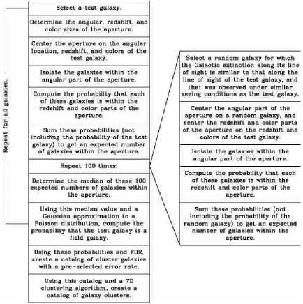
In this section, we present the C4 cluster–finding algo-rithm. Details and tests follow. Many readers will only want a brief explanation of the algorithm and we sug-gest they examine the flowchart of the algorithm given in Figure 2 and read this overview section. For those who desire more details, each step is described in more detail throughout the rest of this section. The applica-tion of the C4 algorithm to the SDSS data is discussed in Section 7.
The C4 algorithm begins by placing each galaxy in a seven dimensional space of right ascension (ra), declina-tion (dec), redshift and four color dimensions (u−g,g−r,
r−i,i−z). On each such target galaxy, we then perform the following steps:
1. We place an aperture around each target to only include galaxies in a specified range of ra, dec, and redshift. We then measure the probability that ev-ery galaxy within this spatial aperture has colors equal to the target galaxy. The probabilities are summed to obtain a “number count”.
2. Using the target galaxy’s spatial and color ature, we then select 100 random galaxies and per-form step (1). These 100 random locations pro-vide a “number count” distribution for the target galaxy.
3. Using the number count distribution, we compute the probability of obtaining at least the observed number count around the original target galaxy. By definition, target galaxies with low probabilities will be in clustered regions.
4. We repeat this exercise for all (‘target’) galaxies in our sample and then rank all the target galaxy probabilities obtained from step 3.
5. Using the false discovery rate algorithm (FDR; Miller et al. 2001c), we determine a threshold in probability below which target galaxies are re-moved; our threshold choice typically results in the eradication≃90% of all galaxies. The galaxies that remain are called “C4 galaxies”. By construction, these reside in high density regions with neighbors that possess similar colors.
6. We determine the local surface density around all C4 galaxies, using only the C4 galaxies, We then rank order these measured densities and locate C4 cluster centers as peaks in this density field.
In summary, the C4 algorithm is a semi-parametric implementation of adaptive kernel density estimation. The key difference of our approach, compared to pre-vious color-based cluster–finding algorithms, is that we do not attempt to model either the colors of the cluster galaxies (e.g., Gladders & Yee 2000, Goto et al. 2002) or the properties of clusters (e.g., Kepner et al. 1998; Postman et al. 1996; Kim et al. 2002). Instead, we only demand that the colors of nearby galaxies are similar to those of the target galaxy. In this way we are sensitive to a diverse range of cluster and group types e.g., our algorithm would detect a cluster dominated by a “blue” population of galaxies (see Figure 22).
2.1. Defining the 7-dimensional Search Aperture
Every target galaxy in the dataset has a uniquely de-fined location in a 7-dimensional data–space. For exam-ple, the position of theithgalaxy is defined as:
ri= [rai,deci, zi, miu−mig, m i g−m
i r, m
i r−m
i i, m
i i−m
i z],
(1) where mi
X are the five passband Petrosian magnitudes
from the SDSS PHOTO version 5.4 data reductions (typ-ically abbreviatedu, g, r, i, z). Nok–corrections are used herein.
To look for clusters in this 7-dimensional data–space, we need to define a search aperture. Clearly the size of this aperture will have an effect on the types of clusters we find in this data–space. We begin by using a projected radius that is fixed in comoving coordinates, and specifies the ra and dec aperture surrounding the target galaxy. The exact cosmological model used makes little difference over the redshift range we examine here, (z∼0.1). This aperture can be tuned to find the size that optimizes completeness and purity in the mock galaxy catalogs.
We next define the redshift (or line–of–sight) dimen-sion of the C4 search aperture. For the spectroscopic SDSS sample, all galaxies have known redshifts and we simply place az-constraint around the target galaxy. For the SDSS photometric sample, one would need estimated redshifts or else this constraint must be dropped entirely. We have chosen to convert redshift to co-moving distance under an assumed model, but one could also simply let the length of the redshift dimension vary with redshift.
Finally, we must define the color part of our search aperture. The size of the four color dimensions will be driven by the well-established intrinsic color-magnitude relation (CMR) seen in clusters (see Figure 1) and the expected errors on the SDSS magnitudes. The CMR is known to have a linear relationship with a small nega-tive slope (with increasing magnitude) and small scatter (Bower et al. 1992). Therefore, the size of the “color-box” should be set to capture the full range of colors in the CMR, from the brightest to the faintest cluster galaxies in any given cluster in our data. We addition-ally include the known statistical (1σ) uncertainties in the individual galaxy magnitudes. For the SDSS main galaxy spectroscopic sample, these errors are minimal (less than 0.1% at mr = 17.7). We sum in quadrature
these statistical errors and also a systematic uncertainty via:
δCxy= q
σ2
Fig. 2.—Flow chart describing the algorithm
whereσ2
xy(stat) is the observed error for the two
magni-tudes (x, y), summed in quadrature. Hereσ2
xy(sys) is a
measure of the inherent scatter in the CMR (see below). Therefore, for each i galaxy the size of the color box is given by,
δCi= [δCi
ug, δCigr, δCiri, δCiiz]. (3)
We have used the Petrosian magnitudes reported by the SDSS throughout, as it is better suited for the anal-yses of galaxies in the SDSS spectroscopic sample (see Stoughton et al. 2001). However, our final cluster catalog is robust against the use of Petrosian versus model mag-nitudes. We do not apply evolutionary or k–corrections to our data, as we are looking for galaxies clustered in both position and color around another galaxy: for a given redshift and color of a galaxy, any excess of neigh-boring galaxies with similar colors should occur indepen-dent of any evolutionary effects and k–corrections.
Once we have defined the search aperture around a tar-get galaxy, we then “count” the number of neighboring galaxies within that aperture. To do this, we demand
that any neighboring galaxy fit exactly within the spa-tial part of the aperture (ra, dec, and redshift) as these dimensions are accurately known.
In the color dimensions, we allow for uncertainties in both the color box of the target galaxy and the individual colors of surrounding galaxies. Specifically, we replace the color boxes with Gaussians having widths specified by Equation (4), which “softens” the sides of the 4-d color box. We also treat the errors on the individual galaxies as Gaussians. We then measure the the joint probability that any galaxy falls within the color box of the target galaxy. We then sum these probabilities for all neighboring galaxies and report this as the “number count” of neighboring galaxies.
2.2. Building the Count Distributions
above. We allow for the fact that our algorithm can be run on the SDSS photometric data, in which case the seeing conditions and galactic extinction can have a large effect on the selection function of the SDSS pho-tometric sample. The random galaxies can be selected such that they have the same seeing and reddening as the target galaxy. However, on the complete SDSS spec-troscopic sample, we ignore this constraint. From these 100 randomly chosen locations in the data, we construct a distribution of counts for the 7-d aperture of the target galaxy. So long as we expect no more than half of the galaxies to be in clustered environments (i.e., have higher counts with respect to the mean), the medians of these distributions are robust descriptors of the distributions.
2.3. Determining Probabilities
By this stage, we have defined a unique aperture for the target galaxy. We have measured the number of neigh-boring galaxies within its aperture and built a count dis-tribution from 100 random locations at the same red-shift of the target galaxy. We then ask the question: how likely is the observed neighboring galaxy count given the distribution of neighboring galaxy counts for a spec-ified 7-d aperture? The exact form of the distribution of neighboring galaxy counts depends on the number of counts measured. For example, in the photometric SDSS data, where there are millions of galaxies, the distribu-tions of neighboring galaxy counts is Gaussian. However, in the spectroscopic data, the count distributions can sometimes be small and Poissonian. As a compromise, we adopt the Gaussian approximation to the Poisson. In order to justify the basis of Poissonian statistics, we need to meet the following requirements in the count distribu-tion; i)the count within an aperture of zero volume is zero, ii) each of the 100 randomly chosen counts must be independent,iii)the count values depend only on the size of the aperture,iv)the aperture size does not change when building the count distributions, and v) no two counts come from the same location. Requirementsi,ii,iv andvare already met in our algorithm, whileiiirequires that the randomly selected points have an underlying count distribution that is also random. This, of course, is not true for all galaxies, as galaxies are known to clus-ter, and galaxies within clusters have a higher neighbor count than those in the field. However, if a majority of the randomly selected galaxies are “field-like”, i.e., less clustered then the older elliptical population in clusters and groups, then we can expect iii to hold. At worst, this assumption produces a small bias by slightly raising our probabilities, resulting in a loss of statistical power (which would affect the C4 completeness), and so our Poisson assumption is a conservative one.
The Gaussian approximation to the Poisson distribu-tion has the convenient feature that the width of the Gaussian is equal to the square root of the mean of the Poisson distrubution. Thus, when we build the count distributions based on the 100 random locations, we only need to calculate the median, which then fully describes the Gaussian approximation. Thus, the probablility that a target galaxy looks like a field galaxy is determined solely from the count around the target and the median of the counts around the 100 random locations.
2.4. Repeat
Once the above steps are performed on the first target galaxy, we then repeat for all galaxies in sample. This is conducted in no specific order. Once we have looped over the entire sample, every galaxy has a probability that it is a “field galaxy”. These probablities are ranked so that a threshold can be applied to separate the cluster galaxies from the field galaxies.
2.5. Choosing a Threshold
Miller et al. (2001c) present a new thresholding tech-nique known as the False Discovery Rate (FDR) origi-nally devised by Benjamini and Hochberg (1995). This technique allows one to choose a statistically meaning-ful threshold, in the sense that the fraction of false pos-itive detections over the total number of detections is controlled. We apply the techniques discussed in Miller et al. here. Briefly, this involves choosing a priori the maximum fraction of acceptable false discoveries (α) one is willing to tolerate. The p-values (probabilities) are rank–listed (from lowest to highest) and a line of slope
αdrawn. Where the two lines intersect for the first time defines the threshold one must use to guarantee the frac-tion of false discoveries (see Miller et al. 2001c and Hop-kins et al. 2002 for some examples). After applying the FDR technique, all galaxies above the threshold are called “cluster-like” or “C4” galaxies and are then used to identify C4 cluster centers.
We test our probability model and whether our FDR threshold can separate “field” and “cluster-like” galax-ies on a galaxy-by-galaxy level. In Figure 3, we show the distribution of median counts for the count distribu-tions around all galaxies in the mock SDSS catalog (solid line), compared to the individual counts around galax-ies (dash line). We have split our sample into “field-like” and “cluster-“field-like” as described above. Note that the counts around “cluster-like” galaxies are significantly higher than around “field-like” galaxies. Also note that the median counts of the field distributions, and also the counts around “field-like” galaxies, are similar and Poisson. This shows that the medians of the random distributions are representative of “field-like” galaxies. This justifies our use of the median to represent the random distributions, and that the probability thresh-old (discussed below) cleanly separates “field-like” and “cluster-like” galaxies.
2.6. Identifying the clusters
The C4 algorithm works by identifying galaxies clus-tered in a positional and color space. Once the 7-d aper-ture and threshold are defined, galaxies with low proba-bilities of being field-like (as defined by random positions on the sky) are identified as clustered C4 galaxies (10% of all galaxies using our fiducial parameters). We then find centers of the clumps of C4 galaxies, and call these C4 clusters. The algorithm (to this point) does not de-fine the galaxy membership of the clusters (see Section 5).
Fig. 3.—We show the counts from the field based on the median of 100 random locations for each galaxy (solid) and counts around each specific galaxy (dotted). On the left we show for “field-like” galaxies, while on the right we show “cluster-like” galaxies. Notice that “cluster-like” galaxies have more neighbors than the median of the field.
Fig. 4.—Projected galaxy distribution of the simulations before (left) and after (right) the C4 algorithm is run and a threshold is applied to eliminate field-like galaxies.
∆z= 0.02. The nearest neighbor distances are ordered from the smallest to largest, and the C4 galaxy with the smallest sixth nearest neighbor distance is assigned as the center of the first C4 cluster. We then exclude all C4 galaxies from this list out to a projected radius corresponding to 15 times the background density of C4 galaxies centered on this first cluster. This choice of en-hancement is arbitrary. However, this same overdensity is used when examining the real data or the mock cata-logs. We have checked to make sure that the distribution of neighbor distances is the same in both the real SDSS data and in the mock galaxy catalog. We then move to the next highest density C4 galaxy that is not within any other C4 cluster and repeati.e., the C4 galaxy now with the smallest sixth nearest neighbor distance becomes the center of the second cluster and so on. The iterations are terminated when all C4 galaxies are assigned to clus-ters or the local densities fall below the threshold. These initial centers are then peaks in the C4 galaxy surface over-densities.
This process is shown visually in Figures 4 and 5. We investigated other methods for finding the C4 cluster cen-ters (e.g., “friends–of–friends” algorithm etc.), and find this method to be the best in terms of accuracy, com-pleteness, and purity when compared to the actual halo catalog.
During this process, if there are fewer than three C4 neighbors around any cluster center, we exclude it as a possible cluster. Likewise, if we determine that less than 10% of all galaxies in an 1h−1Mpc aperture around the
cluster are classified as C4 galaxies, we exclude it (the number of clusters excluded due to this criteria is less
Fig. 5.—The C4 galaxies, as in Figure 4 (right), with the dark matter halo positions overplotted (red squares). The halos have masses greater than 4.5×10¹³
h−1
M⊙.
than 2% of the total found). Finally, we exclude any clus-ter that has less than eight members within 1h−1Mpc so
that we may measure a reliable velocity dispersion. We note that these exclusions imply that C4 completeness (see Section 4) is lower than it could be, since these ex-cluded systems could often be real systems.
2.7. Other Algorithm Considerations
2.7.1. Survey Edges
[image:7.612.371.532.266.450.2]2.7.2. The Magnitude Limit
The current incarnation of the catalog is run on ap-parent magnitude limited surveys. The SDSS spectro-scopic Main sample was targeted using galaxies brighter than mr = 17.77, while the Luminous Red Galaxy
(LRG) sample includes additional elliptical-type galax-ies to mr = 19.5. While technically this is an input
parameter that could be tuned, we instead consider the effect on completeness, purity, and total number of clus-ters after a single limit is chosen. When measuring the cluster properties (see Section 5), we apply an absolute magnitude limit as well.
3. A MOCK SDSS GALAXY CATALOG
One advantage of the C4 catalog over many previous cluster catalogs is our use of realistic cosmological N-body simulations to refine the algorithm and to deter-mine the completeness and purity of the catalog. Since the C4 algorithm is highly dependent on clustering in both spatial and color space, any mock galaxy catalog must have relations between galaxy color and density that mimic the those found in real data. Similarly, the luminosity functions of the mock catalogs and the data must be similar. Simple bias schemes which produce a population of galaxies above some luminosity cut (e.g., Cole et al 1998) will not produce the information we need to find clusters. Mocks created from more detailed semi-analytic models of galaxy formation (e.g., Kauffmann et al. 1999 and Eke et al. 2004) do produce colors and luminosities; unfortunately at this stage none of these models are yet producing galaxies with properties that nearly enough reproduce those seen in the SDSS data. The mock catalog we use here thus takes a very empiri-cal approach, in which we aim to populate a dark matter simulation with galaxies whose properties (especially, the luminosity and color distributions as a function of envi-ronment) closely match those seen in SDSS data. The method for creating these catalogs is described briefly in Wechsler (2004) and in detail in Wechsler (2005, in preparation, hereafter W05); here we just give a rough outline. A complementary approach, using conditional luminosity functions constrained by galaxy clustering, has been developed by Yang et al. (2004).
The W05 catalogs are constructed using the distribu-tion of dark matter in the ΛCDM Hubble Volume sim-ulation. The simulation follows 109 particles of mass
2.25×10¹²h−1solar masses in a periodic cubical volume
with side length 3h−1Gpc, in a flat Λ CDM universe with
Ωm= 0.3,σ8= 0.9, andh= 0.7. We use a subset of the
MS sky survey output described by Evrard et al. (2002) which mimics the collection of data on the past light cone of an observer located at the center of the volume. We only look at halos more massive than 4.5×10¹³h−1 solar
masses (see below). The large size of the simulation al-lows the creation of a full-sky survey out to a depth of
zmax = 0.57, and thus can also be used to test cluster finding algorithms that use only the SDSS photometric data and extend to higher redshift.
Briefly, the algorithm for creating the W05 catalogs consists of constraining the relation between local dark matter density and luminosity in the r-band, such that the mock galaxies match the luminosity-dependent two-point correlation function measured in the SDSS data (Zehavi et al. 2004). We then measure local galaxy
den-sity in the r-band, for both the data (see Gomez et al. 2003) and the simulation, and assign the colors of real SDSS galaxies to mock galaxies that have similar lumi-nosities and local galaxy densities. All relevant details of these new simulations are presented in W05, including the prescriptions used to assign galaxy properties to each dark matter particle and the extensive tests performed on these simulations to ensure they closely mimic the real data.
The mass resolution of the simulation allows us to include galaxies brighter than about 0.4 L⋆, and to
resolve halos more massive than 4.5 ×10¹³h−1 solar
masses. Therefore, these simulations can only resolve bright galaxies in intermediate–to–massive clusters of galaxies, e.g., a cluster like the Coma Cluster would contain about 500 galaxies in these mock SDSS cata-logs. This makes them well-suited to the brighter (and more massive) galaxies in the SDSS spectroscopic sample (which is what we use in this work), which only includes dimmer galaxies at the lowest redshifts z < 0.05. As discussed above, we place a constraint on any C4 clus-ter that there be at least eight galaxies within 1h−1Mpc
of the cluster centers. For halos at the minimum well-resolved mass in the simulation, only 1% have fewer than eight galaxy members, so nearly all are intrisically de-tectable by the C4 algorithm. This indicates that these simulations allow us to reliably estimate the complete-ness of our catalog over the full mass range of interest, but higher resolution simulations will be required to fully characterize the purity of the smallest C4 systems.
Another advantage of using the HV simulation is that we can directly relate any detected clusters in these mock SDSS catalogs to the measured halo masses discussed by Jenkins et al. (2001) and Evrard et al. (2002). In other words, we can directly relate the observables (e.g., veloc-ity dispersions and summed total cluster optical lumi-nosities) to the dark matter halos used by Jenkins et al. (2001) for constructing the cosmological mass function. There is no ambiguity in the definition of mass between the theoretical models and the observables.
Since the real data will contain photometric errors, we have added errors to each mock galaxy magnitude. How-ever, we note that for the spectroscopic sample, the SDSS Petrosian (1976) magnitude errors are tiny (the largest fractional errors are<0.1% in ther-band). As described in Section 2.1, the size of the colbox is at least an or-der of magnitude larger than the errors on the colors. Thus, this step is not necessary for the spectroscopic data. However, when the full photometric SDSS sam-ple is used (to mr = 22), the photometric errors can in
fact dominate the color-box. Therefore, we have built in this mechanism at this stage. We note that we use the true SDSS errors when the algorithm is run on the real SDSS data. In the mock catalogs, we use the median ob-served error for galaxies in the SDSS main galaxy sample (see Strauss et al. 2002). Our results are insensitive to changes (<50%) in the value of this constant error.
The mock galaxy catalog is complete down to an ab-solute magnitude of Mr =−19.6, which corresponds to mr = 19.2 at z = 0.17 (which is the highest redshift
cluster we find in the real data). We apply an apparent magnitude limit of mr≤17.7 to the SDSS mock catalog
limit is applied and the errors are added, we are able to run the exact same C4 algorithm on the mock galaxy catalogs and identify clusters as outlined in Section 2. For this work, we have used a volume that is larger and more contiguous than the SDSS DR2. However, edge ef-fects are handled identically in the data as they are in the mock catalogs (see Section 2.7.1). While we have not applied the SDSS targeting algorithm, in Section 7.1 we study this issue in detail and find that the effect on completeness and purity is small.
4. COMPLETENESS, PURITY, AND TUNING THE C4
ALGORITHM
We use the SDSS mock galaxy catalogs to test the C4 algorithm, fine tune the choice of parameters, and mea-sure the completeness and purity of the catalog (i.e., the selection function). We do this by running the C4 algo-rithm on the mock galaxy catalog, and comparing the found C4 clusters to the known halos from Evrard et al. (2002). To make the comparison, we apply a matching algorithm to associate C4 clusters with halos. We have investigated several prescriptions for matching these two datasets and have found that our matches are robust against the details of the matching algorithm. Here, we present results based on matching a dark matter halo with any C4 cluster within a projected distance corre-sponding to one virial radius and within ∆z = 0.005. We discuss this matching in more detail in Section 4.2. To estimate purity, we match clusters to any simulated halo within the estimatedr200of the “observed” C4 clus-ter, while for the completeness measurements we match each “observed” C4 cluster to the nearest dark matter halo within ∆z = 0.005 and the projected r200 of the halo.
This method for matching allows for multiple matches. In other words, when measuring completeness, multiple C4 clusters can be matched to one HV halo, and similarly when measuring purity, multiple halos can be matched to a single C4 cluster. There are many ways to deal with this problem. For instance, when multiple halos match to one C4 cluster, we could take the most massive halo as the fiducial match. Or we could take the halo that has the most similar luminosity to the C4 cluster, or any other method. We have chosen to simply take the match that is closest in separation on the sky (and within ∆z = 0.005). We have investigated a few of the other methods we mentioned and find no clear winner. The C4 algorithm finds fewer clusters in the mock catalog than there are real HV halos (i.e., the C4 algorithm is never 100% complete). As seen and discussed in the following sections, this completeness drops with halo mass such that the C4 algorithm can miss up to 50% of the halos at masses∼5×10¹³h−1solar masses. This means that
there will always be more multiple halo matches to the C4 clusters than vice versa. On average, 50% of the C4 clusters have multiple halos within ∆z= 0.005 andr200
while only 5% of halos have multiple C4 clusters within those same constraints.
After the matching is done, we will plot the cumulative quantity:
Purity(Lr) =
Number(> Lr) C4 Matched to Halos
Number(> Lr) C4 Clusters Found
(4)
Completeness(M200) = Num(>M200) Halos Matched to C4 Num(>M200) Total Halos
(5) whereM200is the mass within a radius that is 200 times the critical density andLris the summed luminosities of
the cluster member galaxies as defined in detail in Sec-tion 5. Since completeness is defined against the “true” halos from the mocks, we plot completeness versus halo mass. On the other hand, purity is measured from the point of view of the measured clustered catalog, and so purity is plotted against the observable: optical luminos-ity. It is important to keep in mind that the high mass (or high luminosity) systems are rare, and so the purity and completeness measurements can be noisy in these regimes.
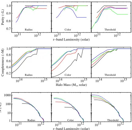
In Figure 6 (left), we present the completeness and purity of the mock C4 catalog as a function of differ-ent radii for the search aperture: 500,1000,2000, and 6000h−1kpc. In this figure, the other dimensions of the
search aperture are fixed at the final values as discussed below. A radius of 500h−1kpc (black) appears to be too
small, as it significantly lowers the completeness of our sample for all but the most massive systems (although it does produce the purest sample). However, larger search-radii make little difference to the completeness or purity of the algorithm. The highest completeness and purity occur when a co-moving radius of 1h−1Mpc is used (the
red line).
We varied the redshift dimension of the 7-d box to be a co-moving length of 25,50,100,200h−1Mpc. The size
of the aperture in the redshift direction must be large enough to allow for significant (and unknown) peculiar velocities of galaxies within massive clusters of galax-ies and therefore, our 3-dimensional positional aperture is shaped like a narrow cylinder. Using these tests, we find that our final cluster catalog is independent of the length of the line-of-sight aperture. We attribute this to the fact that there are not many clusters or groups that lie directly along the line-of-sight that also have similar global colors. Alternatively, one could argue that by not using k–corrections for our SDSS colors, we have already accounted for the redshift dimension in the “color-box”. We set the redshift dimension of the search aperture to 50h−1Mpc.
In the middle panel of Figure 6, we show the complete-ness and purity for the mock SDSS catalog as a function of the “color-box” size, holding constant the spatial part of the search aperture. We examine only the effect of changingσxy(sys), usingσug(sys) =γ×0.15, σgr(sys) = γ×0.12, σri(sys) = γ×0.1, and σiz(sys) = γ×0.1.
These values represent reasonable widths for the color-magnitude relation, decrease with increasing wavelength (as indicated in Figure 1), and are motivated by the re-sults of Goto et al. (2002). However, we note that our al-gorithm is not attempting to model the color-magnitude relation. Thus, we allow the color-box size to be a free parameter in our algorithm by varyingγas 1,2,4,6. We then use the mock galaxy catalogs to tune this variable. We note that the median of σxy(stat) = 0.02 for our
data changes very little over our magnitude-range (re-call, these are the bright galaxies in the spectroscopic SDSS data). Thus, σxy(sys) is the dominant term in
Equation (4).
10
11
10
12
0.7
0.8
0.9
1.0
Purity (<L)
10
11
10
12
r−band Luminosity (solar)
10
11
10
12
Radius Color Threshold
10
14
10
15
0.2
0.4
0.6
0.8
1.0
Completeness (>M)
10
14
10
15
Halo Mass (M
200solar)
10
14
10
15
Radius Color Threshold
10
11
10
12
1
10
100
1000
N (>L)
10
11
10
12
r−band Luminosity (solar)
10
11
10
12
[image:10.612.96.528.173.597.2]Radius Color Threshold
dimension produces a very pure, but highly incomplete (black) sample, as was the case for the smaller radial aperture. As we increase the size of the color box, we increase the completeness, while decreasing the purity. For the final algorithm, we chooseγ = 4 which has the highest completeness (forM ≥1014M
⊙ systems), while still maintaining a high level of purity.
In the right panel of Figure 6, we show the complete-ness and purity of the C4 sample as a function of the FDR threshold. We varyα from 0.05, 0.10, 0.15, 0.20, and 0.50. We note that our least conservative thresh-old (α= 0.5) produces the highest completeness, but at the expense of purity. By lowering the FDR threshold, one simply increases the number of C4 galaxies being se-lected, but these extra galaxies either increase the detec-tion likelihood of clusters already detected at higher FDR thresholds, or form a background which decreases the purity. Changing the threshold by a factor of four only improves the C4 completeness for M200 ≤1×10¹⁴M
⊙ systems by∼10%, but at the price of decreasing the pu-rity for such systems by 10%. Based on this, we choose
α= 0.1 (the red line) which provides both a high purity and completeness. This is preferred over maintaining a higher completeness (e.g. α= 0.5), as it provides users of the C4 catalog the confidence to pick and choose real clusters for any scientific analyses. Also, as we discuss in section 4.2, gains in the measured completeness are as much a result of random matches as they are from a more efficient algorithm. When this final threshold is ap-plied, approximately 90% of all galaxies are excluded as not being in color and spatially clustered environments. In Figure 7, we show purity, completeness, and num-ber for clusters in shells of equal volume, increasing in redshift from black to red to green to blue to vio-let, covering redshift ranges of [0.03,0.075], [0.075,0.093], [0.093,0.107], [0.107,0.118], [0.118,0.128] respectively. As with Figure 6, these panels use the mock galaxy cata-logs. However, unlike Figure 6 whose clusters numbered in the many hundreds, these smaller volume bins contain ∼100−200 clusters and so the results are noisier. As ex-pected, completeness decreases with increasing redshift, but varies little out toz= 0.107 for all masses. Beyond that, completeness drops steeply. Purity is fairly con-stant (to within 10%) over all redshift ranges, however the lowest redshift bin is the purest. The C4 catalog is
>90% complete and>95% pure for systems more mas-sive than∼2×10¹⁴M
⊙(or brighter than∼3×10¹¹L⊙) and out to a redshift ofz∼0.12. In the bottom panel of Figure 7, we see that the number function is mostly de-pendent on the completeness in each redshift shell. The most complete bin (lowest redshift) shows the highest number of low luminosity (or mass) clusters. As com-pleteness dwindles with redshift (and mass), the number of found halos decreases similarly. The excess ofN(> L) in Figure 7 (bottom) for the highest redshift bin (violet) is due to a single bright, massive halo in the simulations.
4.1. The Strength of Color Clustering
We have run a series of tests to determine whether our choice of all four colors is necessary for our stated goals (high purity and known completeness) compared to using just a subset of these colors. Specifically, we ran the C4 algorithm using each of the four colors separately, as well as using subsets of the colors, e.g., g−r andr−i, but
notu−gor i−z.
In Figure 8 (left), we show how the purity of the C4 catalog changes as we add in more color information. The highest purity comes from using all four colors. As expected, the reddest color selectioni−zdoes well (even though thez-band magnitudes have greater photometric uncertainties). Combining two colors does reasonably well and is better than only using a single color. We conclude that the choice of four colors gives us our high-est purity.
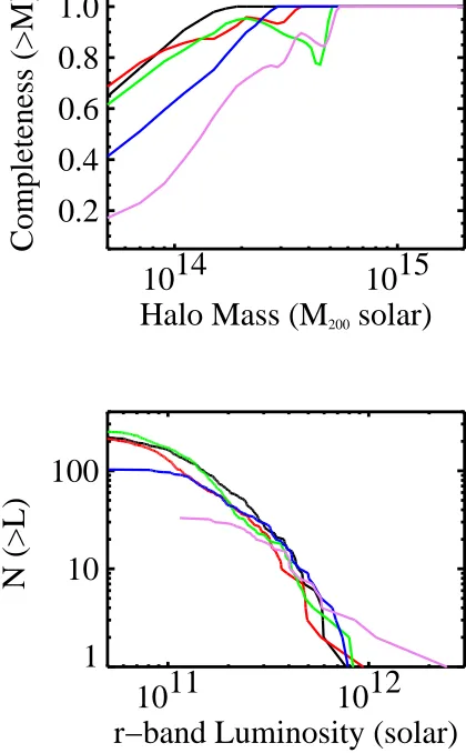
We next examine the completeness as a function of our color choices. In Figure 8 (right), we present com-pleteness as a function of halo mass for the same color selections as used above in the purity case (solid lines). The highest purity case (using all four colors) results in the lowest completeness. At first glance, it appears that the use of a single or double color criteria produces better results, with 10% higher completeness than the four color case. This is, however, misleading: the higher formal completeness is in fact entirely due to random matches (the dotted lines in Figure 8). For example, at M = 1×10¹⁴M
⊙, the completeness increases from
∼ 70% for the four color criteria to 80% for the sin-gle i−z color selection. At the same time, the random matches (described below) increase by 10% and the pu-rity decreases by ∼10%. In other words, the single and double color criteria have approximately twice as many detected “clusters” as the four color criteria, producing a much greater chance for random matches. Of course, as seen in Figure 8, a larger fraction of these detected “clusters” are spurious. We discuss in more detail the random matches in the next section.
As a final test, we should mention here that we exper-imented with shuffling the colors of the galaxies in the mock catalogs, while keeping their positions fixed, and re-ran the C4 algorithm. We found only a few of the clos-est richclos-est clusters, which again demonstrates the power of color clustering in 4–dimensions.
4.2. Random Matches
These first results raise the issue of the number of ran-dom matches one would expect given any sample. We quantify random matches by selecting the same number of clusters as found by the C4 algorithm, but centered on random galaxies in the mock catalog. For example, if we find 934 clusters in the mock catalog using the algo-rithm, we select 934 galaxies at random from the same mock catalog and use them as our cluster centers. We then match these with the dark matter halo catalog us-ing the same criteria as before. We show the “complete-ness” from a sample of randomly-placed cluster centers as the dotted line in Figure 8 (right). As expected, the “completeness” of the random matches monotonically in-creases with cluster mass because the number of clusters as a function of mass monotonically decreases, while the number of matches remains fixed. In other words, for a fixed number of random positions, a greater fraction of rare rich clusters is recovered compared to the numerous poor clusters.
10
11
10
12
r−band Luminosity (solar)
0.7
0.8
0.9
1.0
Purity (<L)
10
14
10
15
Halo Mass (M
200solar)
0.2
0.4
0.6
0.8
1.0
Completeness (>M)
10
11
10
12
r−band Luminosity (solar)
1
10
100
[image:12.612.206.416.326.665.2]N (>L)
Fig. 7.—The completeness, purity, and number of halos brighter thanLrfor equal volume shells, each at increasing redshift. The shells
1011 1012 r−band Luminosity (solar) 0.75
0.80 0.85 0.90 0.95 1.00
Purity
1014 1015
Halo Mass (M200 solar)
0.0 0.2 0.4 0.6 0.8 1.0 1.2
[image:13.612.95.531.277.487.2]Completeness
Fig. 8.—Left: Purity of the C4 catalog as a function of different color selections. The black-line (highest purity) comes from using all four colors. In both panels, the green, turquoise, orange, and red correspond to using onlyu′−g′, g′−r′, r′−i′, andi′−z′only. The
purple corresponds to using bothg′−r′andr′−i′ only. Right: Measured completeness of clusters found using the C4 algorithm (solid
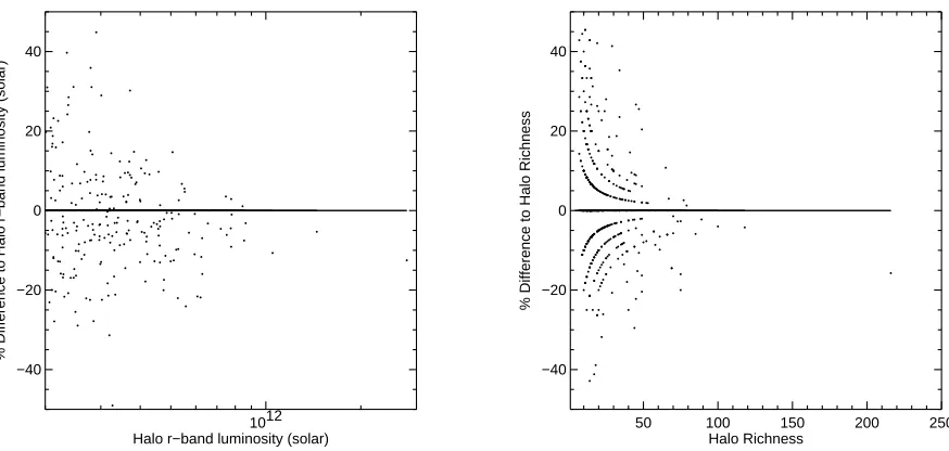
we recover the halo observables after we find C4 clusters in the mock catalogs and match to the halos. We show difference between the recovered and the “true” summed optical luminosities and richnesses (see Section 5). These figures show that we recover the true observables to typ-ically within 20%.
Inherent in these analyses is our ability to match halos to the C4 clusters. Keep in mind that halos from simula-tions are themselves messy, non-spherical systems whose boundaries are dependent on the exact identification al-gorithm (Lacey & Cole 1994; White 2002). The halo sample we employ is based on a spherical overdensity approach. Details of the finding algorithm and the resul-tant halo samples are published in Evrard et al. (2002). A more detailed exploration of matching clusters to dark matter halos is presented in W05.
4.3. The Final C4 Algorithm Parameters
The parameters of our final algorithm are: (1) an aper-ture on the sky corresponding to 1h−1Mpc projected at
the redshift of the target galaxy; (2) a redshift box cor-responding to a fixed co-moving±50h−1Mpc around the
target galaxy ; (3) a 4-d color-box of width specified by Equation (5) and
[σsys ug , σ
sys gr , σ
sys ri , σ
sys
iz ] = [0.6,0.48,0.4,0.4] (6)
We apply a probability threshold that results in no more than 10% contamination.
These parameters have been tuned to produce a clus-ter catalog with the highest possible purity and similarly high completeness. We note that Figure 6 shows that the measured purity and completeness are very robust to modest changes in the tunable parameters. The algo-rithm is demonstrably robust.
4.4. Summary of C4 Catalog Purity and Completeness
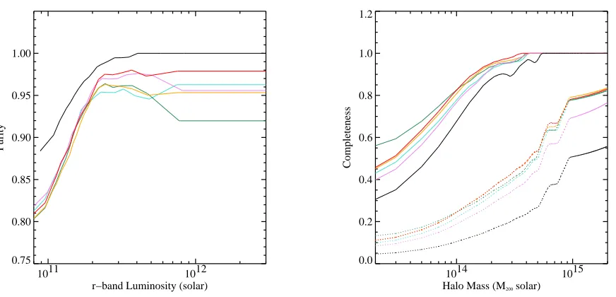
In Figure 10 we present the final purity and complete-ness of the C4 catalog based on our optimal parameter choices as discussed above (over all redshifts). Recall, pu-rity is defined to be the percentage of systems detected in the mock SDSS catalog, using the C4 algorithm, and matched to any dark matter halo (more massive than 4.5×10¹³) in the HV simulation. We also measure the
purity as a function of velocity dispersion, using only those clusters which contain ten or more galaxies. We find that our C4 catalog is 100% pure for such systems and thus do not present this result in a figure.
As one can see in Figure 10 (left–solid line), the purity of the C4 sample remains at 100% for the most massive systems, dropping down to ∼ 90% for the remainder. The C4 catalog is more than 99% pure for luminosities larger than 3×10¹¹L
⊙. The high purity of the C4 catalog is a direct product of our search for clusters in a high– dimensional space.
In Figure 10 (right–solid line), we also show the com-pleteness of the C4 algorithm, as a function of halo mass (M200), as selected from the mock SDSS catalog. This figure demonstrates that the C4 catalog remains more than 90% complete for systems with M200>∼2×10¹⁴M⊙. Below this mass the catalog becomes progressively more incomplete and is only 55% complete at M200 ≃ 1×
1014M
⊙. The completeness is only 30% for the lowest mass systems probed here (M200≃2×10¹³M⊙).
4.5. Questions about the C4 Methodology
We address here three common questions raised about the C4 approach. These are:
1. Why focus on the photometric data in the C4 al-gorithm, when the redshifts (i.e., the 3-d positions in redshift-space) are known?
2. Why use all four SDSS colors (u−g,g−r,r−i,i−z)? Why not use the spectra of the galaxies, instead of the broad-band filters?
3. Does the algorithm miss clusters with younger stel-lar populations?
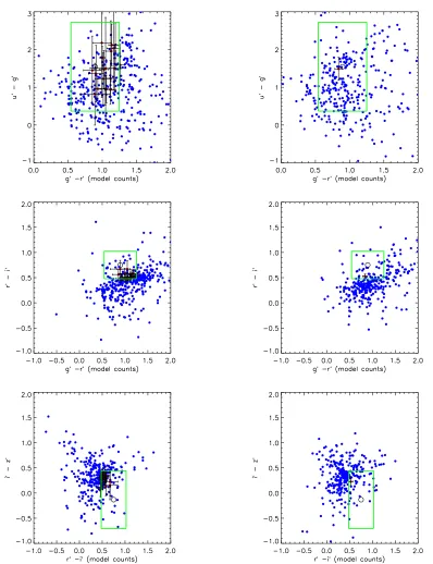
In Figure 11, we address the first question and demon-strate the power of using the color information in addi-tion to the spatial coordinates. Here, we show the projec-tion of the SDSS 7–dimensional search aperture (4 color and 1 spatial coordinates) onto the different color–color planes for both a cluster and field region. In Figure 11, we have placed the same size physical aperture over two galaxies: one in a clustered environment (left panels in Figure 11) and the other in a field-like environment (right panels in Figure 11). The galaxy on which the color-color plots are centered is the target galaxy and is identified by the open circle.
The blue dots are all galaxies within the spatial part of the search aperture. Visually, one might be able to detect the spatial clustering by noticing that there are more galaxies in the clustered versus the field en-vironment (388 versus 327) The red dots are galaxies that lie within the color-box in all three figures. Note that this “color box” (green) is the same, in location and size, for both the cluster and field environments. The over-density of galaxies in the clustered environ-ment now becomes much more apparent — there are 19 cluster galaxies (red dots) that have both similar po-sitions and colors to the target galaxy, while there re-mains only one galaxy (with similar colors and position) in the field-like environment. This process increases the signal–to–noise of the cluster over-density (compared to the field over-density) from 388/327 to 19/1, so that the slight over-density in the three–dimensional position– space becomes an extreme over-density in the much sparser seven–dimensional data–space used here. Fig-ure 11 demonstrates the elimination of projection effects and the strength of color in galaxy clustering. It also demonstrates the enhancement of the overdensities one can achieve by using positions andcolors in our cluster-ing algorithm,
1012 Halo r−band luminosity (solar) −40
−20 0 20 40
% Difference to Halo r−band luminosity (solar)
50 100 150 200 250
Halo Richness −40
−20 0 20 40
[image:15.612.93.530.68.276.2]% Difference to Halo Richness
Fig. 9.— Left: The percentage difference between the measured cluster optical luminosity compared to the “true” halo luminosity.
Right: Same asLeftexcept for the Richness. The method of measuring luminosities and richnesses is described in Section 5. For the C4 clusters, we use the centroid of the found cluster, while for the halos we use the centroid as reported in the halo catalog.
1011
1012
r−band Luminosity (solar) 0.75
0.80 0.85 0.90 0.95 1.00
Purity
1014
1015
Halo Mass (M200 solar)
0.0 0.2 0.4 0.6 0.8 1.0 1.2
[image:15.612.95.527.333.537.2]Completeness
Fig. 10.—The final measured purity and completeness of our C4 catalog using the mock SDSS catalog. The solid is measured before the fiber collision algorithm is applied (see Text). The dotted line shows the effect missing galaxies due to fiber collisions.
the smallest photometric errors, which results in a tight “red sequence” in the g−r, r−i color–color plane (see Figure 1). Finally, the z passband is useful as it pro-vides the best measurement of the old stellar population for these low redshift galaxies and is the least affected by galactic reddening. The larger errors on the z–band photometry do not compromise the C4 algorithm as we take the observed errors into account when constructing the 7–dimensional search aperture.
With regard to using the spectra instead of the SDSS colors, we note that the five SDSS passbands (u, g, r, i, z) cover a larger wavelength range than the spectra. The central wavelengths of the SDSS photometric filters are 3550˚A, 4770˚A, 6230˚A, 7620˚A, 9130˚A respectively, cov-ering a wavelength range from≃3300˚Ato one micron. In comparison, the spectra only cover a wavelength range
of 3900˚A to 9100˚A. From a computational standpoint, using the spectral data instead of the photometric colors would require working in a many thousand-dimensional data–space. Even with a million galaxy spectra, such a high–dimensional data–space would be severely under-populated, leading to statistical problems in finding any clustering in the data. In summary, the 7–dimensional data–space discussed herein is very effective for our task of finding clusters and groups of galaxies, as the dimen-sionality is sufficient to eradicate projection effects while remaining manageable in size.
Fig. 11.— The different SDSS color-color planes for an example cluster galaxy (left) and a randomly chosen field galaxy (right). The blue dots are all galaxies within the spatial part of our search box (ra, dec, redshift), while the red dots are those galaxies which are also with the color part of our 7–dimensional search aperture (shown in green).
match the environmental trends seen in the data. Thus, the colors allow us to achieve our goals of maximizing completeness and eliminating projection effects, as tested against the mock galaxy catalogs.
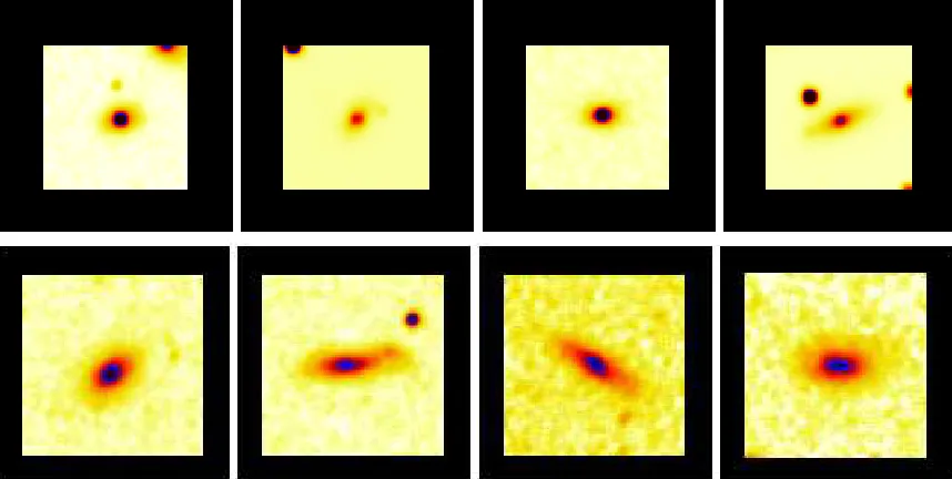
To address the final question, in Figure 12 we present two groups of galaxies found by the C4 algorithm which possess very different galaxy properties. The first group of galaxies in Figure 12 (top) contains galaxies which ap-pear redder, and more elliptical–like — as expected in a typical group of galaxies. The second group in Figure 12 (bottom) contains much bluer, diskier galaxies. These
Fig. 12.—We show the images of two sets of four galaxies that are clustered in both position and color. The top four are elliptical galaxies at a redshift of∼0.027 and all lie within a projected distance of 350h−1
kpc. The bottom four are galaxies that are diskier and have a younger stellar population (i.e., they are bluer). The bottom four galaxies are at a redshift of∼0.04 and all lie within a circle that
is 450h−1
kpc in radius. The positions and colors of the galaxies in each of the sets are all very similar and listed in Table 1.
TABLE 1
Galaxy Position and Colors in Figure 12
ra dec redshift u′−g′ g′−r′ r′−i′ i′−z′
Red Galaxies(Top)
219.409 3.946 0.025 5.01 0.67 0.31 0.20 219.481 3.984 0.029 5.38 0.75 0.37 0.22 219.778 3.999 0.027 4.00 0.72 0.37 0.22 219.887 3.925 0.029 4.86 0.56 0.22 0.14
Blue Galaxies (Bottom)
228.312 4.513 0.036 0.89 0.34 0.43 0.29 228.445 4.251 0.041 1.19 0.32 0.42 0.00 228.574 4.064 0.042 1.13 0.29 0.45 0.40 228.277 4.195 0.037 1.09 0.45 0.40 0.12
of spectral types. However, galaxy types are not broadly classified, but bi-modal (spirals or elliptical, star-forming or passive). Thus, to first order, every cluster will con-tain at least 50% of one of the two major types of galaxies and the algorithm will find such color clustering.
5. MEASURED CLUSTER PROPERTIES
For each C4 cluster we measure a set of quantities which include the cluster centroid, the velocity disper-sion, and the summedr-band luminosity. In addition, we characterize the substructure and local large-scale struc-ture of each cluster.
5.1. Cluster Centroids
We measure three different cluster centroids: (1) the peak in the C4 density field, (2) the luminosity weighted mean centroid, and (3) the position of the brightest clus-ter galaxy. Method (1) was discussed in Section 2.6. Method (2) uses all galaxies within 1h−1Mpc of the
ini-tial centroid (Method 1) and within four velocity disper-sions (see next section). We then calculate an r-band luminosity weighted center. Method (3) attempts to
identify the brightest cluster galaxy (BCG). The BCG is taken as the brightest galaxy within 500h−1kpc of the
initial centroid (Method 1), within four velocity disper-sions (see next section), and which has no strong Hα
emission (< 4˚A). We then report the position of the BCG.
The cluster redshift we report is determined via the bi-weighted statistic of Beers et al. (1990). We use only those galaxies within 1h−1Mpc of the initial centroid and
within ∆z = 0.02 of the peak in the redshift histogram as described in the next subsection.
5.2. Velocity Dispersions
To calculate the velocity dispersion of galaxies in our clusters, we perform an iterative technique based on the robust bi-weighted statistic of Beers et al. (1990). Hav-ing defined the sky-positional centroid of each cluster, we construct a redshift histogram of all galaxies (regard-less of their C4 classification) within a projected radius of 1h−1 Mpc. We then search this histogram for a peak
and tentatively identify this peak as the velocity center of the cluster (as a lower limit, this peak must contain at least three galaxies within 1000 km/s of each other). We iterate by only keeping galaxies within 1.5h−1 projected
Mpc of the cluster centroid and within ∆z= 0.02 of the velocity center defined above. We then compute the bi-weighted mean recessional velocity for these galaxies and measure their bi-weighted velocity dispersion, σest
v .
We stress that the above procedure is performed on all available galaxies in the SDSS spectroscopic sample. For consistency, we check that each cluster contains a certain number of C4 galaxies, and reject those clusters where this fraction is below 10% of all galaxies within 1h−1Mpc and ∆z = 0.02. Only a small fraction (2%)
[image:17.612.52.294.363.504.2]the velocity dispersion, consistent with previous limits to get a reliable value (see Collins et al. 1995). Note that most (80%) of our clusters in the real SDSS data con-tain ≥ 20 galaxies with which to measure the velocity dispersion. Clusters which do not meet this criteria are removed from the main sample. To get our final veloc-ity dispersion measurements (σv), we re-calculate it for
each cluster using only galaxies within four times the es-timated velocity dispersion (σest
v ) discussed above. This
is similar to the standard sigma-clipping method used in the literature. The accuracy of these final measurements, which are in the observed reference frame, are discussed below.
5.3. Summed Optical Cluster Luminosity
To calculate the total summedr–band optical luminos-ity for each cluster, we convert the apparent magnitudes of all cluster members into optical luminosities, using the conversions in Fukugita et al. (1996), and sum them. All magnitudes are k-corrected according to Blanton et al. (2003a) and extinction corrected according to Schlegel, Finkbeiner, and Davis (1998). Cluster membership is confined to galaxies within 4σv in redshift–space and a
projected radius of 1.5h−1Mpc on the sky. The SDSS
main galaxy sample is designed to be complete (>95%) to mr = 17.77 and the C4 cluster sample is complete
(>90%) toz= 0.11. Thus, to minimize effects from the SDSS selection function, we use an absolute magnitude limit ofMr<−19.9, which is an apparent magnitude of mr= 17.8 atz≃0.11, when measuring the optical
lumi-nosities. Clusters beyondz= 0.11 will need to have their optical luminosities corrected for this incompleteness.
5.4. Structure Contamination Flag
We define a “Structure Contamination Flag” (SCF) to measure the degree of isolation in redshift–space for each cluster. Specifically, we examine radial varia-tions of the velocity dispersion for each cluster, noting large radial variations from the mean velocity disper-sion. Clusters which are embedded in surrounding large-scale structure can have significant velocity contamina-tion. SCF increases with increasing standard deviations in the velocity dispersion profiles. We calculate the bi-weight velocity dispersion within 500,1000,1500,2000 and 2500h−1kpc radial bins as described above, and
deter-mine the standard deviation. We then assign an SCF based on the ratio of the standard deviation of the dis-persions over the mean of the velocity disdis-persions. We use three bins, SCF = [0,2], in approximating the bot-tom, middle, and top thirds of the distribution of the ratio. A cluster with SCF = 0 has a ratio less than 15% whereas SCF = 2 has a ratio>30%. The sky plot and velocity profile are shown for a real SDSS cluster with a high SCF=2 cluster in Figure 21, 23, and 24. Notice that the velocity dispersion as a function of radius is highly erratic, producing a large standard deviation about the mean. Figures 23 and 24 show two clusters separated by less then two tenths of one degree and ∆z = 0.01. Notice that the velocity dispersion profile increases sys-tematically as the galaxies from the neighboring system are picked up with increasing aperture. These clusters both have SCF = 2. A clusters with SCF = 1 is shown in Figure 22 and with SCF = 0 in 25. Notice here that the velocity dispersion profiles are nearly constant. This
SCF flag does not necessarily quantify the substructure of the main cluster, but rather identifies clusters whose velocity dispersions may be inaccurate because of nearby large-scale structure.
5.5. Dressler-Shectman Statistic
In addition to quantifying the local large–scale struc-ture for each cluster, we can use the Dressler-Shectman substructure statistic to search for local differences in a cluster’s mean recession velocity and velocity dispersion. For each cluster member (within 1.5h−1Mpc and 4σ
v),
we compute a local recession velocity and local velocity dispersion using the ten nearest neighbors to the galaxy which are also within 4σv of the cluster redshift. We
then compute the difference between these local quanti-ties and the mean recession velocity and velocity disper-sion for the whole cluster. The cumulative differences are then used as a measure of the cluster substructure. To compute the significance of this measurement, we shuffle the galaxy velocities within the cluster and repeat the ex-ercise 1000 times. Using these Monte-Carlo realizations, we calculate the probability that the observed cumulative differences would be obtained at random, given the spa-tial positions of the galaxies. A low probability indicates that the substructure is significant. For more details, see Dressler and Shectman (1988) and Oegerle and Hill (2001).
6. SCALING RELATIONS AND THEIR SCATTER Any galaxy cluster catalog will have observables that can be related to the underlying halo dark matter mass. Typically, researchers have used some sort of galaxy num-ber count, i.e., richness (Abell 1958, Yee and Ellingson 2003). While the C4 clusters certainly have galaxy num-ber counts, we also measure the summed r-band lumi-nosity of the galaxies within each cluster. We addition-ally measure a velocity dispersion for all clusters within our spectroscopic data (using 8 or more galaxy mem-bers within a projected radius of 1h−1Mpc and within
four velocity dispersions). In this section, we determine which cluster observables scale best with the halo masses in the mock galaxy catalogs. We stress that this sec-tion does notquantifyany absolute scaling-laws (or their scatter), which requires a detailed analysis of the role of cosmology and of the sensitivity of this scaling to the halo occupation. This will be presented in an upcoming paper. Here, we simply study how the scatter changes as we vary parameters of the cluster finding algorithm and measures of the local foreground/background con-tamination. In short, the scaling relations presented in this section are used solely to guide our choice of the best cluster observable when relating to mass, as qualified by the scatter, and we caution the reader not to use them to draw cosmologically-dependent conclusions.
6.1. Structure Contamination and Velocity Dispersion
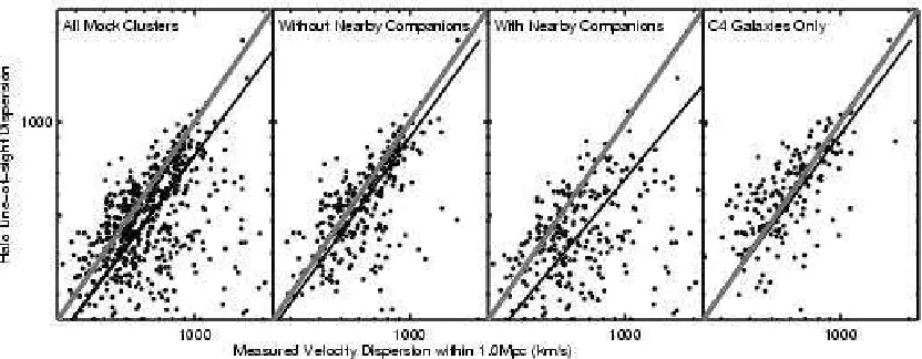
Fig. 13.— Using the mock clusters, we compare our measured velocity dispersions to the line-of-sight velocity dispersions measured directly on the halo-particles in the HV Simulations. The thick grey line is the one-to-one line, while the black line is the best fit when SCF = 0. We use only clusters with 10 or more members within a projected radius of 1h−1
Mpc and within 4σv. The best fit relation
occurs when SCF=0 where the rms scatter is∼15%. 1.0h−1Mpc and within 4σ
v. We find an excellent
one-to-one agreement with ∼15% scatter (using only those mock clusters with SCF = 0. This scatter doubles if we use all clusters. Therefore, the structure contamination flag is essential in recovering the true velocity dispersions of the systems. We also show the comparison when we use only the C4 galaxies to measure the velocity disper-sion. Notice that the C4 galaxies are not strongly af-fected by local structure contamination. However, there are fewer systems with enough (>10) galaxies to measure an accurate dispersion.
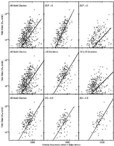
In Figure 14 we present the correlation between halo mass and the measured velocity dispersions of C4 clus-ters in the mock SDSS catalog. We present the best (robust-fit) linear relationship between these two physi-cal quantities. Here, there is also significant asymmetri-cal scatter about this relationship, with many low mass systems possessing an apparently high velocity disper-sion. Part of this asymmetry and scatter is due to the number of galaxies used to measure the velocity disper-sion. In Figure 14 (middle) we split the sample into clusters with less than 25 members and more than 25 members within 1.5h−1Mpc. As expected, clusters with
a larger number of members have higher mass halos, but we also observe that the scatter decreases by∼50% for the regression when only the high-number systems are used. Unfortunately, if we place a cut on the number of cluster members to reduce the scatter in this scaling law, we also constrain ourselves to only the higher mass systems.
As an alternative to using only clusters with the most galaxies for accurate velocity dispersions, we plot in Fig-ure 14 (top row), the relationship betweenM200 and ve-locity dispersion, but now separated on the Structure Contamination Flag (SCF). The scatter in the relation is reduced by a factor of two after we include only those clusters with SCF = 0. Additionally, the scatter is re-duced over the whole mass range of the clusters. This demonstrates that a majority of the scatter in Figure 14 is due to SCF > 0 systems, which by definition have a known companion within 1.5h−1Mpc−1 of the main
cluster. The end result i