An adaptive interface compression method for water entry and exit

An adaptive interface compression method for water

entry and exit

Dominic J. Piro and Kevin J. Maki

University of Michigan

Department of Naval Architecture and Marine Engineering

No. 2013-350

March 2013

Abstract

A common method for the simulation the two-phase flow is the volume of fluid (VOF) method. The VOF method involves the advection of a function with large gradients at the interface between the two phases. One strategy to maintain a sharp interface is to employ an artificial velocity field that is compressive. The current work extends this method to be adaptive, using the compressive velocity only when desirable. The desirability of the compression is defined in terms of the entry and exit of a wedge shaped body. For water entry, interface compression is desirable, while for exit it produces spurious free-surface features. The adaptive compression term is shown to work well for the problem where the wedge enters and then subsequently exits the water.

1

Introduction

Finite-volume computational fluid dynamics (CFD) of free-surface flows can use either interface-tracking or interface-capturing methods. Interface-tracking methods often include deforming the grid to conform with the free-surface boundary. A common interface-capturing method is the volume-of-fluid (VOF) method [1], which is the focus of this paper. This method uses an scalar ↵ to denote the volume fraction of a fluid in each cell, and ranges from 0 to 1. ↵ is known as either the volume fraction or indicator function. The interface between two fluids is represented as the jump from 0 to 1 of ↵(often the ↵= 0.5 contour is used). Thus the issues of advecting a discontinous function occur when using VOF - a stable and monotone method is required that also reduces the smearing of the discontinuity.

and Tryggvason [4] track the free surface with a deforming unstructured grid while solving the fluid equations on a fixed stuctured grid. These are just a few examples of interface-tracking methods. The main difficulties in using interface-interface-tracking methods are the cost of deforming meshes as well as the posibility of the free surface folding onto itself. Interface-capturing schemes do not have these problems and are thus more commonly used for complex free-surface flows.

For interface-capturing, a method to maintain boundedness and sharpness at the same time, called CICSAM (compressive interface capturing scheme for arbitrary meshes), uses the normalized variable diagram (NVD) [5]. The NVD allows for definition of regimes when upwind, downwind, and central di↵erencing provide stable and monotonic advection of the volume fraction. The CICSAM method shows good results advecting a scalar with a step on both structured and unstructured meshes.

A di↵erent high-resolution discretization scheme for VOF is proposed by Walters and Wolgemuth [6]. The bounded gradient maximization (BGM) scheme is introduced which represents face values of the volume fraction as a linear combination of the upwind and downwind cells. The face value is limited to remain in the range [0,1]. The BGM scheme is shown to maintain a less smeared interface than the high-resolution interface capturing scheme of Muzaferija et al. [7].

A bounded compression term is used by Rusche [8] that acheives compression of the interface with an artificial velocity that pushes the volume fraction toward the free surface. This formulation allows for the use of monotonic discretization schemes without the worry about smearing of the interface. The compression term contains an constant coefficient term that allows the user to scale the compression. This artificial velocity formulation is used in the current work.

˘

Strubelj and Tiselj [9] use a two-fluid model instead of a single-fluid model. This model solves separate equations for each fluid and contains a volume fraction for each phase. The paper [9] adds interface-sharpening to the two-fluid model by solving an equation on the volume fraction that acts as an artificial compression. With the interface sharpening, the model is shown to simulate the Rayleigh-Taylor instability well.

An alternative interface-capturing method to VOF is the level set method. In the level set method, the free surface is defined as a iso-contour, or “level set”, of a scalar function (often the distance from the interface). This scalar function is smooth at the interface and thus the issues of VOF regarding advecting a discontinuity do not exist. The major drawback of the level set method is that the basic formulation does not conserve mass. Recently, there has been development of conservative level set methods [10] to alleviate this issue. The conservative level set method is shown to have good results when the grid is fine enough.

0.00 5.00 10.00 15.00 20.00 25.00

0.00 0.03 0.06 0.09 0.12 0.15 0.18

F/(0.5

ρ

V

2 B)

Vt/B C_α = 0 C

α = 1 Zhao (1993) 0 0.5 1 1.5 2 2.5 3 3.5 4 4.5 5

-0.02 0 0.02 0.04 0.06 0.08 0.1 0.12 0.14

F/(0.5

ρ

V

2 B)

Vt/B C_α = 0 C

α = 1

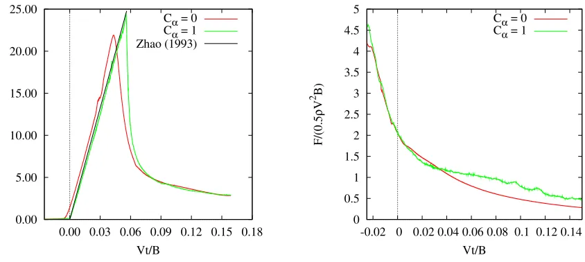
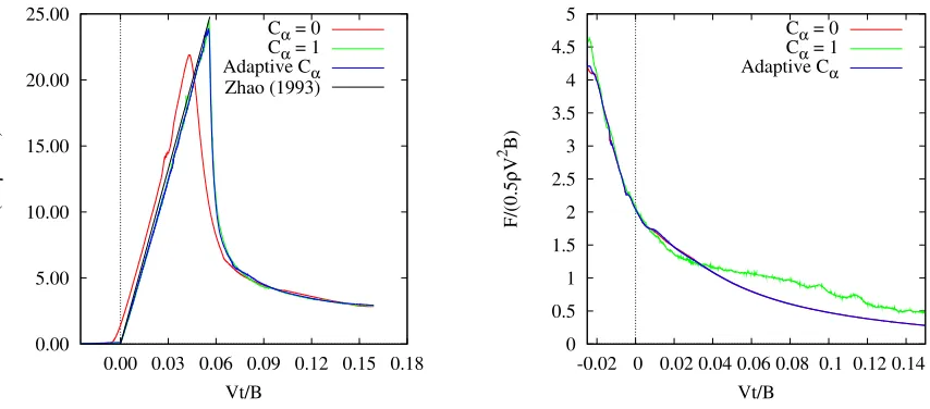
Figure 1: Vertical Force on wedge while entering (left) and exiting (right) the water with and without compression.

2

Motivation

The use of the adaptive compression coefficient has been motivated by the study of the water entry and exit of wedge-shaped bodies. First, Figure 1 shows the usefulness of compression for constant velocity water entry problems (left graph) with the force on a 10 deadrise wedge. Time is non-dimensionalized by the velocity V and the beam B. The force is also non-dimensionalized byV andB, as well as the water density⇢. For the same mesh, the entry force is more accurately predicted when using compression (C↵ = 1). Without compression (C↵ = 0) a layer of air (↵ < 0.5) is trapped along the body, and thus the peak force is lower, the force does not drop as sharply, and the smearing of the interface causes the body to “see” the water before it should arrive. Compression therefore allows for more efficient calculations of entry flows. The results of Zhao and Faltinsen [11] using a boundary element method (BEM) are shown for comparison. The force using C↵ = 1 compares very well to the BEM results, while the results with C↵ = 0 do not compare as well.

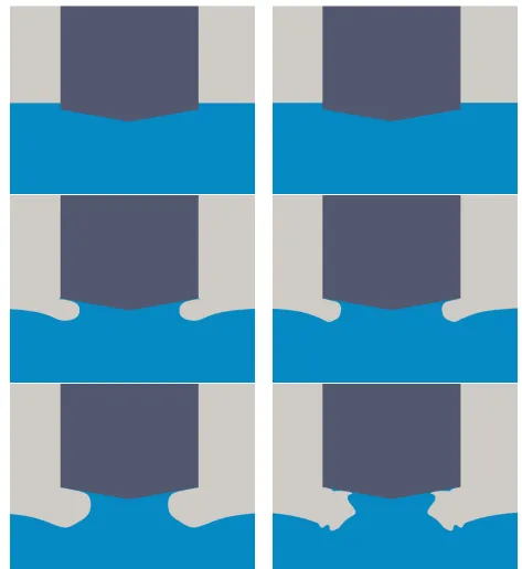
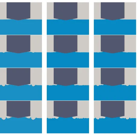
During constant velocity exit calculations using the same mesh as above, compression can result in spurious features in the free surface, as seen Figure 2. The images in the left column do not use interface compression (C↵ = 0), while those in the right column use full compression (C↵ = 1). The free surface remains smooth throughout the calculation without compression. However, with compression, a small perturbation can grow unphysically due to the artificial compressive velocity. Figure 1 (right) shows that the force time series is also smoother when not using interface compression. Note that for this case t= 0 when the calm free surface reaches the chine, and that the vertical force is upwards (positive) because water rushing in to fill the void under the wedge is trapped by symmetry, causing a positive dynamic pressure and thus vertical force, as seen in Piro [12].

and the relative velocity is used to determine the which regime the flow is in.

3

Methodology

3.1

Computational Fluid Dynamics Solver

The open-source computational fluid dynamics library OpenFOAMR is used to solve the

fluid equations of motion. A finite-volume discretization is used with arbitrary Lagrangian-Eulerian (ALE) formulation [13] to allow for moving and deforming grids. The fluid is assumed to be laminar and incompressible. The fluid is governed by the Navier-Stokes equations:

r·~u= 0, (1)

@⇢~u

@t +r·⇢~u~u= rp+r· µ r~u+r~u

T _{+⇢~g, (2)}

where~u is the fluid velocity,⇢and µthe fluid density and dynamic viscosity, andpthe fluid pressure.

The volume fraction is used to determine the fluid properties:

⇢=↵⇢1+ (1 ↵)⇢2, (3)

µ=↵µ1+ (1 ↵)µ2, (4)

where ⇢1 and µ1 are the properties for fluid 1 (e.g. water) and ⇢2 and µ2 are the properties

for fluid 2 (e.g. air). The governing di↵erential equation for↵, from Rusche [8], is

@↵

@t +r·(↵~u) +r·(↵(1 ↵)~ur) = 0, (5)

where~ur is the artificial compressive velocity. The↵(1 ↵) scaling ensures that the artificial velocity only acts near the interface. The alpha equation is discretized (with _JK denoting a numerical derivative inside the brackets):

s

@[↵]

@t {

+q_r· [↵]f( ,S) y+qr· rb[↵]f( rb,S)

y

, (6)

where is volumetric flux and:

rb = (1 ↵)f( r,S) r, (7)

r =C↵~n⇤max|

~n⇤ _|

|S~|2 . (8)

u_rel

Entry Flow:

C > 0

Exit Flow:

C = 0

u_rel

1 0

1 0

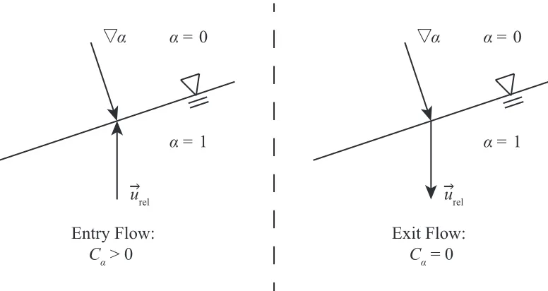
Figure 3: Illustration of calculation of adaptive compression coefficient

3.2

Adaptive Interface Compression

The current work varies the interface compression coeffient with the following equation:

C↵ = max

✓

~

urel·r↵

|~urel||r↵|+✏

,0 ◆

, (9)

where ~urel is the relative fluid velocity to the mesh, calculated as ~urel = ~u ~um, ~um is the

mesh velocity, and✏ is a small number to ensure the denomenator is not zero. This equation sets C↵ to the negative of the cosine of the angle between the gradient of ↵and the relative velocity if the angle is greater then 90 and 0 otherwise. Thus, the range of C↵ is [0,1], where C↵ ⇡ 1 will be seen on entry, and C↵ = 0 on exit of a body from water. Figure 3 illustrates theC↵ calculation process.

4

Results

In this section two studies are shown. The first section uses the entry and exit of a flat plate to further explore the cause of the free-surface instabilities. Then a wedge is used to demonstrate the proposed adaptive compression method. For these studies the densities used are⇢w = 1000 kg/m3 for water and ⇢a= 1 kg/m3 for air.

4.1

Flat Plate Model

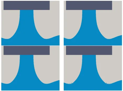
Figure 4: Free-surface profiles at timet = 1 s for fine grids: isotropic (top row) and stretched (bottom row). C↵ = 0 for the left column andC↵ = 1 for the right column.

a coarse version of each grid with 100 cells along the plate and a fine version with 200 cells along the plate are used.

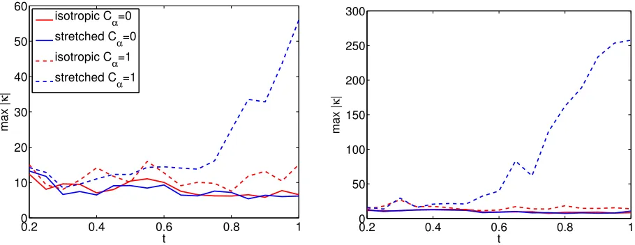
The isotropic grid does not generate the free-surface instabilities with or without interface compression, while the grid with stretching develops the instabilities with compression on. Figure 4 shows the free-surface profile for the fine versions of the isotropic and stretched grids with and without interface compression. The perturbations can be clearly seen at the lowest point on the free-surface for the stretched grid. The maximum free-surface curvature throughout the simulations is shown in Figure 5, with the coarse grids on the left and fine grids on the right. The instabilities are shown through large curvature (corresponding to a small radius of curvature) of the free-surface on the stretched grids. Of note is that the curvature on the stretched grid grows more rapidly for the finer case than the coarser case. Even though on the isotropic grid the curvature is larger with interface compression, it does not appreciably grow during the simulation, signifying that it is not the sole cause of the free-surface instabilities.

0.2 0.4 0.6 0.8 1 0 10 20 30 40 50 60 t max | κ |

isotropic C_α=0

stretched C α=0 isotropic C α=1 stretched C α=1

0.2 0.4 0.6 0.8 1

0 50 100 150 200 250 300 t max | κ |

Figure 5: Maximum free-surface curvature for coarse (left) and fine (right) grids.

vertical direction. As stretching in the vertical direction can be desirable to develop efficient meshes, motivation is provided for disabling compression when the instabilities are likely to occur.

4.2

Wedge Model

The test body in the following work is a wedge (See Figure 6). The wedge has beam B

between the chines (transitions from the sloped wedge to vertical walls) and deadrise angle . For this work, the deadrise angle is set to be = 10 . The beam is used with velocity to non-dimensionalize time and the vertical force on the wedge. The discretization schemes are backward di↵erencing for @/@t, linear-upwind for _r·(⇢~u~u) and vanLeer for _r·(↵~u).

The wedge entry and wedge exit problems described above are used to ensure that the proposed adaptive compression method works as expected. The adaptive compression coef-ficient is compared to constant coefcoef-ficients of 0 (no compression) and 1 (full compression). Figure 7 shows that the force using the adaptive compression follows the full compression for entry (left plot) and no compression for exit (right plot). This shows that the adaptive com-pression term behaves as expected - activating comcom-pression during entry and deactivating compression during exit.

The adaptive interface compression is used to solve the problem of a wedge that enters and and then subsequently exits the water. For the wedge entry and exit problem, the body is given a parabolic trajectory as in [14, 15]. A case in which the chines of the wedge are not wetted and has more violent exit flow is selected. The force on the wedge is shown in Figure 8 and free surface evolution in Figure 9. For this case, time is non-dimensionalized byt0, the time between the keel reaching the calm free surface and the time of zero velocity

(maximum immersion).

B

Chine

Figure 6: Wedge model used in this study

0.00 5.00 10.00 15.00 20.00 25.00

0.00 0.03 0.06 0.09 0.12 0.15 0.18

F/(0.5

ρ

V

2 B)

Vt/B C_α = 0 C_α = 1 Adaptive C_α Zhao (1993)

0 0.5 1 1.5 2 2.5 3 3.5 4 4.5 5

-0.02 0 0.02 0.04 0.06 0.08 0.1 0.12 0.14

F/(0.5

ρ

V

2 B)

Vt/B

C_α = 0

C_α = 1

Adaptive C_α

-35 -30 -25 -20 -15 -10 -5 0 5 10 15 20

0 0.5 1 1.5 2

F/(0.5

ρ

V

2 ave

B)

t/t₀

C_α = 0

C_α = 1

Adaptive C_α

Figure 8: Force on wedge entering and exiting the water with and without compression and with adaptive compression.

smoother, and the free surface has fewer perturbations away from the body.

The entry and exit calculations without compression do not give acceptable results with this mesh. A layer of air is trapped along the wedge, inhibiting the formation of the jet. When the wedge is exiting, the smeared interface near the body splits apart and results in a much di↵erent flow than with the adaptive compression. Also, without compression, a disturbance in the force is seen just before t/t0 = 2.

5

Conclusions

Acknowledgments

The authors would like to gratefully acknowledge the support of a grant from the US Office of Naval Research, Award # N00014-10-1-0301 and # N00014-11-1-0846, under the technical direction of Ms. Kelly Cooper.

References

[1] C. W. Hirt and B. D. Nichols. Volume of fluid (VOF) method for the dynamics of free boundaries. Journal of Computational Physics, 39:201–225, 1981.

[2] S Chen, D. B. Johnson, P. E. Raad, and D Fadda. The surface marker and micro cell method. International Journal for Numerical Methods in Fluids, 25(7):749–778, 1997.

[3] Samuel W.J. Welch. Local simulation of two-phase flows including interface tracking with mass transfer. Journal of Computational Physics, 121(1):142 – 154, 1995.

[4] Salih Ozen Unverdi and Gr´etar Tryggvason. A front-tracking method for viscous, in-compressible, multi-fluid flows. Journal of Computational Physics, 100(1):25 – 37, 1992.

[5] O. Ubbink and R.I. Issa. A method for capturing sharp fluid interfaces on arbitrary meshes. Journal of Computational Physics, 153(1):26–50, 1999.

[6] D. Keith Walters and Nicole M. Wolgemuth. A new interface-capturing discretization scheme for numerical solution of the volume fraction equation in two-phase flows.

In-ternational Journal for Numerical Methods in Fluids, 60(8):893–918, 2009.

[7] S. Muzaferija, M. Peric, P. Sames, and T. Schellin. A two-fluid Navier-Stokes solver to simulate water entry. InTwenty-Second Symposium on Naval Hydrodynamics, pages 638–651. Washington, DC, 1998.

[8] Henrik Rusche.Computational fluid dynamics of dispersed two-phase flows at high phase fractions. PhD thesis, Imperial College, London, 2002.

[9] L. ˘Strubelj and I. Tiselj. Two-fluid model with interface sharpening. International

Journal for Numerical Methods in Engineering, 85(5):575–590, 2011.

[10] Tony W. H. Sheu, C. H. Yu, and P. H. Chiu. Development of level set method with good area preservation to predict interface in two-phase flows. International Journal for Numerical Methods in Fluids, 67(1):109–134, 2011.

[11] R. Zhao and O. Faltinsen. Water entry of two-dimensional bodies. Journal of Fluid Mechanics, 246:593–612, 1993.

[12] D.J. Piro and K.J. Maki. Water exit of a wedge-shaped body. In 27th _{Workshop on}

Water Waves and Floating Bodies, Copenhagen, Denmark, April 2012.

[13] Hrvoje Jasak. Dynamic mesh handling in openfoam. In 47th _{AIAA Aerospace Sciences}

[14] D.J. Piro and K.J. Maki. Hydroelastic wedge entry and exit. In 11th _{International}

Conference on Fast Sea Transportation, Honolulu, Hawaii, USA, Spetember 2011.