A trust region spectral method for large scale systems of nonlinear equations

R E S E A R C H

Open Access

A trust region spectral method for

large-scale systems of nonlinear equations

Meilan Zeng

_{and Guanghui Zhou}

*_{Correspondence:}

[email protected] 2_{School of Mathematical}

Sciences/Information College, Huaibei Normal University, Huaibei, 235000, China

Full list of author information is available at the end of the article

Abstract

The spectral gradient method is one of the most effective methods for solving large-scale systems of nonlinear equations. In this paper, we propose a new trust region spectral method without gradient. The trust region technique is a globalization strategy in our method. The global convergence of the proposed algorithm is proved. The numerical results show that our new method is more competitive than the spectral method of La Cruzet al.(Math. Comput. 75(255):1429-1448, 2006) for large-scale nonlinear equations.

MSC: 65H10; 90C06

Keywords: nonlinear equations; trust region; spectral method; large-scale problem

1 Introduction

In this paper we introduce a trust region spectral method for solving large-scale systems of nonlinear equations

F(x) = , ()

whereF:Rn_→Rn_{is continuously differentiable and its Jacobian matrixJ(x)∈R}n×n_is sparse,nis large. Large-scale systems of nonlinear equations have been widely applied in many aspects, such as network-flow problems, discrete boundary value problems, etc.

Many algorithms have been presented for solving the large-scale problem (). Bouaricha et al.[] proposed tensor methods. Bergamaschiet al.[] proposed inexact quasi-Newton methods. The above methods need to calculate the Jacobian matrix or an approximation of it at each iteration. La Cruz and Raydan [] introduced the spectral method for (). The method uses the residual±F(xk) as a search direction and the trial point at each iteration is xk–λkF(xk), whereλkis a spectral coefficient.λksatisfies the Grippo-Lampariello-Lucidi (GLL) line search condition

f(xk+λkdk)≤ max

≤j≤M–f(xk–j) +αλk∇f(xk)

T_{dk, ()}

where f(x) = _F(x), M is a nonnegative integer, α is a small positive number and dk=±F(xk). This method also requires one to compute a directional derivative or a very good approximation of it at every iteration. Later La Cruzet al.[] proposed a spectral

method without gradient information, which uses a nonmonotone line search globaliza-tion strategy

f(xk+λkdk)≤ max

≤j≤M–f(xk–j) +ηk–αλ 

kf(xk), ()

where_kηk≤η<∞. Meanwhile, conjugate gradient techniques have been developed for solving large-scale nonlinear equations (see [–]). In fact, spectral gradient, BFGS quasi-Newton, and conjugate gradient methods can solve large-scale optimization problems and systems of nonlinear equations (see [–]). The advantage of spectral methods is that the storage of certain matrices associated with the Hessian of objective functions can be avoided.

The purpose of this paper is to extend the spectral method for solving large-scale sys-tems of nonlinear equations by using the trust region technique. For the traditional trust region methods [], at each iterative pointxk, the trial stepdkis obtained by solving the following trust region subproblem:

minqk(d) such that d ≤k, ()

whereqk(d) =_F(xk) +J(xk)d.

The above trust region methods are particularly effective for small to medium-sized systems of nonlinear equations; however, the computation and storage loads can greatly increase with increased dimension.

For the large-scale problems of nonlinear equations, we useγkIas an approximation of J(xk). At each iterative pointxkin our method, the trial stepdkis obtained by solving the following subproblem:

minqk(d) = 

Fk+γkd

 _{such that d ≤}

k, ()

whereγkis the spectral coefficient andFk=F(xk). The classic quasi-Newton equation is

Bk+dk=yk. ()

In (), we left-multiplyyT

k and setBk+=γk+I, it follows that

γk+=

yT kyk

yT_kdk, ()

wheredk=xk+–xkandyk=Fk+–Fk.

The paper is organized as follows. Section  introduces the new algorithm. The con-vergence theory is presented in Section . Section  demonstrates preliminary numerical results on test problems.

2 New algorithm

the actual reduction as

Aredk(dk) =f(xk) –f(xk+dk), ()

the predict reduction as

Predk(dk) =qk() –qk(dk). ()

Now we present our algorithm for solving (). The algorithm is given as follows.

Algorithm 

Step . Choose <η<η< , <β<  <β,> . Initializex, <<¯. Setk:= .

Step . EvaluateFk, ifFk ≤, then terminate.

Step . Solve the trust region subproblem () to obtaindk.

Step . Compute

rk=Aredk(dk)

Predk(dk). ()

Ifrk<η, thenk=βk, go to Step . Otherwise, go to Step .

Step . xk+=xk+dk;

k+=

⎧ ⎨ ⎩

min{βk,¯}, ifrk≥η,

k, otherwise.

Computeγk+by (). Setk:=k+ , go to Step .

3 Convergence analysis

In this section, we prove the global convergence of Algorithm . The global convergence of Algorithm  needs the following assumptions.

Assumption A

() The level set ={x∈Rn_|f(x)≤f(x

)}is bounded.

() The following relation holds:

[Jk–γkI]TFk=Odk.

Then we get the following lemmas.

Lemma . |Aredk(dk) –Predk(dk)|=O(dk_).

Proof By () and (), we have

Aredk(dk) –Predk(dk) = qk(dk) –f(xk+dk)

= 

 Fk+γkdk

_{–Fk+Jkdk+Odk}

≤[γkI–Jk]TFkdk+Odk =Odk

.

This completes the proof.

Similar to Zhang and Wang [], or Yuanet al.[], we obtain the following result.

Lemma . If dkis a solution of(),then

Predk(dk)≥

γkFkmin

k,Fk

|γk|

. ()

Proof Sincedkis a solution of (), for anyα∈[, ], it follows that

Predk(dk) =  

Fk–Fk+γkdk

≥ 



Fk–Fk–γk αk

γkFkγkFk 

=αkγkFk–  α



kγk. ()

Then we have

Predk(dk)≥ max

≤α≤

αkγkFk–  α



kγk

≥ 

γkFkmin

k,Fk

|γk|

. ()

The proof is complete.

Lemma . Algorithmdoes not circle between Stepand Stepinfinitely.

Proof If Algorithm  circles between Step  and Step  infinitely, then for alli= , , . . . , we havexk+i=xk, andFk>, which implies thatrk<η,k→.

By Lemmas . and ., we have

|rk– |=|Aredk(dk) –Predk(dk)|

|Predk(dk)| ≤

O(dk₎

kγkFk →

. ()

Therefore, forksufficiently large

rk≥η, ()

this contradicts the fact thatrk<η.

Proof By the definition of Algorithm , we have

rk≥η> . ()

This implies

f(xk+)≤f(xk)≤ · · · ≤f(x).

Therefore,{xk} ⊂ . According tof(xk)≥, we know that{f(xk)}converges. The following theorem shows that Algorithm  is global convergent under the conditions of Assumption A.

Theorem . Let AssumptionAhold,{xk}be generated by Algorithm.Then the algorithm either stops finitely or generates an infinite sequence{xk}such that

lim

k→∞Fk= . ()

Proof Assume that Algorithm  does not stop after finite steps. Now we suppose that () does not hold, then there exist a constantε>  and a subsequence{kj}satisfying

Fkj ≥ε. ()

LetK={k|Fk ≥ε}.

LetS={k|rk≥η}. Using Algorithm  and Lemma ., we have

k∈S

f(xk) –f(xk+)

≥

k∈S

η·Predk(dk)≥

k∈K η·

ε|γk|  min

k, ε

|γk|

.

By Lemma ., we know that{f(xk)}is convergent, then

k∈S

η·

ε|γk|  min

k, ε

|γk|

<∞.

Thus, we have

k∈S

k<∞. ()

From Steps - of Algorithm  it follows that

k+≤k, () for allk∈/S, thus () means

k∈K

Therefore there existsx∗such that

lim k→∞xk=x

∗_{. ()}

By (), we havek→, which implies

Predk(dk)≥ε|γk|  k

for all sufficiently largek. The fact that|Aredk(dk) –Predk(dk)|=O(dk_{) indicates that}

lim k→∞rk= ,

which shows that, for sufficiently largekandk∈K,

k+≥k.

The above inequality contradicts (). Thus, the conclusion follows.

4 Numerical experiments

In this section, the recent spectral method in [] is called Algorithm . We report results of some numerical experiments of Algorithms  and . We choose  test functions as follows (see [, , ]).

Function  The trigonometric function

fi(x) =n– n

j=

cosxj+i( –cosxi) –sinxi, i= , , . . . ,n.

Initial guess:x= –(_n, . . . ,_n)T.

Function  The discretized two-point boundary value problem

F(x) =Ax+(x),

whenAis then×ntridiagonal matrix given by

A= ⎛ ⎜ ⎜ ⎜ ⎜ ⎜ ⎜ ⎜ ⎝

 – –  –

. .. ... ... –  –

–  ⎞ ⎟ ⎟ ⎟ ⎟ ⎟ ⎟ ⎟ ⎠ ,

and= ((x),(x), . . . ,n(x))Twithi(x) =sinxi– ,i= , , . . . ,n.

Function  The Broyden tridiagonal function

fi(x) = ( – xi)xi–xi–– xi++ , i= , , . . . ,n,

x=xn+= .

Initial guess:x= (–, . . . , –)T.

Function  The Broyden banded function

fi(x) =xi + x_i+  – j∈Ji

xj( +xj), i= , . . . ,n,

Ji=j:j=i,max(,i–ml)≤j≤min(n,i+mu), ml= ,ml= . Initial guess:x= (–, . . . , –)T.

Function  The variable dimensioned function

fi(x) =xi– , i= , , . . . ,n– ,

fn–(x) =

n–

j=

j(xj– ),

fn(x) = _n–

j=

j(xj– ) 

.

Initial guess:x= ( –_n,  –_n, . . . , )T.

Function  The discrete boundary value function

f(x) = x+ .h(x+h+ )–x,

fi(x) = xi+ .h(xi+ih+ )–xi–+xi+, i= , , . . . ,n– ,

fn(x) = xn+ .h(xn+nh+ )–xi–,

h=  n+ .

Initial guess:x= (h(h– ),h(h– ), . . . ,h(nh– ))T.

Function  The logarithmic function

fi(x) =ln(xi+ ) –xi

n, i= , , , . . . ,n.

Initial guess:x= (, , . . . , )T.

Function  The strictly convex function

fi(x) =exi_{– , i= , , , . . . ,n.}

Function  The exponential function

f(x) =ex–– ,

fi(x) =iexi–_{–xi, i= , , . . . ,n.}

Initial guess:x= (_nn_–,_nn_–, . . . ,_nn_–)T.

Function  The extended Rosenbrock function (nis even). Fori= , , . . . ,n/,

fi–(x) = 

xi–xi–

,

fi(x) =  –xi–.

Initial guess:x= (–., , . . . , –., )T.

Function  The singular function

f(x) =

 x  +  x  ,

fi(x) = – x  i + i x  i +  x 

i+, i= , , . . . ,n– ,

fn(x) = – x  n+ n x  n.

Initial guess:x= (, , . . . , )T.

Function  The trigexp function

f(x) = x+ x–  +sin(x–x)sin(x+x),

fi(x) = –xi–exi––xi+xi

 + x_i+ xi++sin(xi–xi+)sin(xi+xi+) – ,

i= , , . . . ,n– ,

fn(x) = –xn–exn––xn+ xn– .

Initial guess:x= (, , . . . , )T.

Function  The extended Freudentein and Roth function (nis even). Fori= , , . . . ,n/,

fi–(x) =xi–+

( –xi)xi– 

xi– ,

fi(x) =xi–+

( +xi)xi– 

xi– .

Initial guess:x= (, , . . . , , )T.

Function  The Troech problem

f(x) = x+hsinh(x) –x,

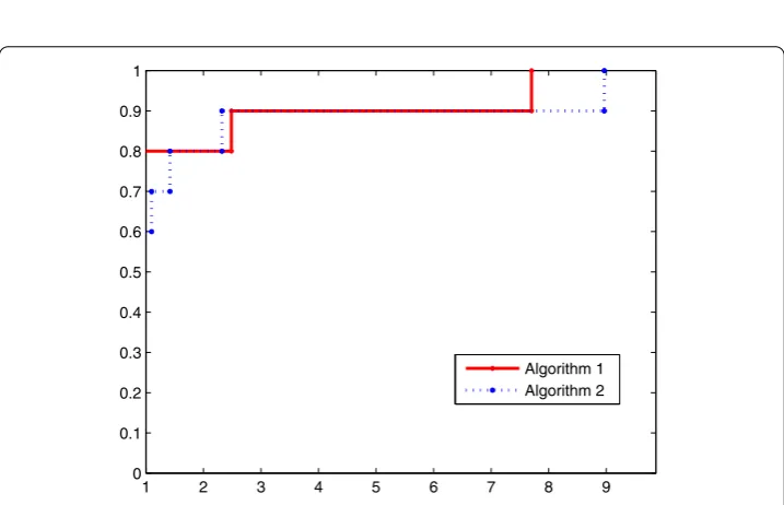
Figure 1 Performance profiles of the total number of iterations of two algorithms (n= 100).

Figure 2 Performance profiles of the total number of iterations of two algorithms (n= 1,000).

fn(x) = xn+hsinh(xn) –xn–,

h= 

n+ , = .

Initial guess:x= (, , . . . , )T.

In the experiments, the parameters are chosen as= ,¯ = ,= –,η= .,

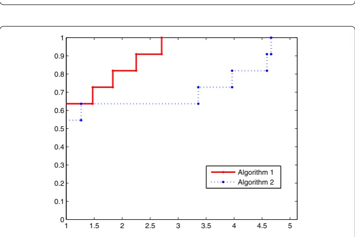
Figure 3 Performance profiles of the total number of iterations of two algorithms (n= 10,000).

Figure 4 Performance profiles of the CPU time of two algorithms (n= 100).

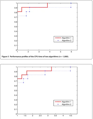
To show the performance of two algorithms, we use the performance profile proposed by Dolan and Moré []. The dimensions of  test functions are , ,, ,. Accord-ing to the numerical results, we plot two figures based on the total number of iterations and the CPU time, respectively.

Figure 5 Performance profiles of the CPU time of two algorithms (n= 1,000).

Figure 6 Performance profiles of the CPU time of two algorithms (n= 10,000).

Competing interests

The authors declare that they have no competing interests.

Authors’ contributions

The two authors contributed equally to the writing of this paper. All authors read and approved the final manuscript.

Author details

1_{College of Mathematics and Statistics, Hubei Engineering University, Xiaogan, 432000, China.}2_{School of Mathematical}

Sciences/Information College, Huaibei Normal University, Huaibei, 235000, China.

Acknowledgements

We thank the reviewers and the editors for their valuable suggestions and comments which improve this paper greatly. This work is supported by the Science and Technology Foundation of the Department of Education of Hubei Province (D20152701) and the Foundations of Education Department of Anhui Province (KJ2016A651; 2014jyxm161).

References

1. La Cruz, W, Jose, MM, Marcos, R: Spectral residual method without gradient information for solving large-scale nonlinear systems of equations. Math. Comput.75(255), 1429-1448 (2006)

2. Bouaricha, A, Schnabel, RB: Tensor methods for large sparse systems of nonlinear equations. Math. Program.82(3), 377-400 (1998)

3. Bergamaschi, L, Moret, I, Zilli, G: Inexact quasi-Newton methods for sparse systems of nonlinear equations. Future Gener. Comput. Syst.18(1), 41-53 (2001)

4. La Cruz, W, Raydan, M: Nonmonotone spectral methods for large-scale nonlinear systems. Optim. Methods Softw.

18(5), 583-599 (2003)

5. Li, Q, Li, D: A class of derivative-free methods for large-scale nonlinear monotone equations. IMA J. Numer. Anal.31, 1625-1635 (2011)

6. Yuan, GL, Zhang, MJ: A three-terms Polak-Ribiè-Polyak conjugate gradient algorithm for large-scale nonlinear equations. J. Comput. Appl. Math.286, 186-195 (2015)

7. Yuan, GL, Meng, ZH, Li, Y: A modified Hestenes and Stiefel conjugate gradient algorithm for large-scale nonsmooth minimizations and nonlinear equations. J. Optim. Theory Appl.168, 129-152 (2016)

8. Barzilai, J, Borwein, JM: Two-point step size gradient methods. IMA J. Numer. Anal.8(1), 141-148 (1988)

9. Birgin, EG, Martinez, JM, Raydan, M: Inexact spectral projected gradient methods on convex sets. IMA J. Numer. Anal.

23(4), 539-559 (2003)

10. Dai, YH, Zhang, H: Adaptive two-point stepsize gradient algorithm. Numer. Algorithms27(4), 377-385 (2001) 11. Dai, YH: Modified two-point stepsize gradient methods for unconstrained optimization. Comput. Optim. Appl.22(1),

103-109 (2002)

12. Raydan, M: The Barzilai and Borwein gradient method for the large scale unconstrained minimization problem. SIAM J. Control Optim.7(1), 26-33 (1997)

13. Yuan, GL, Lu, XW, Wei, ZX: BFGS trust-region method for symmetric nonlinear equations. J. Comput. Appl. Math.230, 44-58 (2009)

14. Yuan, YX: Trust region algorithm for nonlinear equations. Information1, 7-21 (1998)

15. Zhang, JL, Wang, Y: A new trust region method for nonlinear equations. Math. Methods Oper. Res.58(2), 283-298 (2003)

16. Yuan, GL, Wei, ZX, Liu, XW: A BFGS trust-region method for nonlinear equations. Computing92(4), 317-333 (2011) 17. Moré, JJ, Garbow, BS, Hillstrom, KE: Testing unconstrained optimization software. ACM Trans. Math. Softw.7(1), 17-41

(1981)

18. Wang, YJ, Xiu, NH: Theory and Algorithm for Nonlinear Programming. Shanxi Science and Technology Press, Xi’an (2004)