R E S E A R C H
Open Access
An intermixed iteration for constrained
convex minimization problem and split
feasibility problem
Kanyanee Saechou
1and Atid Kangtunyakarn
1**Correspondence: [email protected] 1Department of Mathematics, Faculty of Science, King Mongkut’s Institute of Technology Ladkrabang, Bangkok, Thailand
Abstract
In this paper, we first introduce the two-step intermixed iteration for finding the common solution of a constrained convex minimization problem, and also we prove a strong convergence theorem for the intermixed algorithm. By using our main theorem, we prove a strong convergence theorem for the split feasibility problem. Finally, we apply our main theorem for the numerical example.
MSC: 46N10; 47H09; 74G60
Keywords: Constrained convex minimization problem; Split feasibility problem; Variational inequality
1 Introduction
LetHbe a real Hilbert space with inner product·,·and norm · . LetCbe a nonempty, closed, and convex subset of a real Hilbert spaceH.
We denote the fixed point set of a mappingT byF(T). Fixed point theory can be ap-plied to variational inequality problems, equilibrium problems, split feasibility problems, optimization problems, etc. These problems are encountered in various fields such as en-gineering, physics, game theory, and economics.
A mappingTofCinto itself is callednonexpansiveif
Tx–Ty ≤ x–y, ∀x,y∈C.
In mathematics, conventional optimization problems arise in the process of making a trading system more effective and are usually stated in terms of minimization problems. In this paper, we give a new iteration for solving two constrained convex minimization problems.
Convex constrained minimization problem is popular and very important to various branches in physics, engineering and economics, e.g., to find the minimum travel dis-tance or to find the lowest cost. Consider the constrained convex minimization problem as follows:
minimizef(x) :x∈C, (1)
where f :C→Ris a real-valued convex function. If f is (Fréchet) differentiable, then the gradient-projection algorithm (GPA) generates a sequence {xn}using the following
recursive formula:
xn+1=PC
xn–λ∇f(xn)
, ∀n≥0, (2)
or more generally,
xn+1=PC
xn–λn∇f(xn)
, ∀n≥0, (3)
where both in (2) and (3) the initial guessx0is taken fromCarbitrarily, and the parameters,
λorλn, are positive real numbers satisfying certain conditions. The convergence of the
algorithms (2) and (3) depends on the behavior of the gradient∇f. In fact, it is known that if∇f isα-strongly monotone andL-Lipschitz with constantsα,L≥0, then the operator
T:=PC(I–λ∇f) (4)
is a contraction; hence, the sequence{xn}defined by the algorithm (2) converges in norm
to the unique minimizer of (1). However, if the gradient∇f fails to be strongly monotone, the operatorTdefined by (4) could fail to be contractive; consequently, the sequence{xn}
generated by the algorithm (2) may fail to converge strongly [1]. If∇f is Lipschitz, then the algorithms (2) and (3) can still converge in the weak topology under certain conditions [2–4].
The variational inequality problem is to find a pointu∈Csuch that
v–u,Au ≥0, ∀v∈C. (5)
We denote the set of solutions of the variational inequality byVI(C,A). Many models of variational inequalities are used in practice, including a mathematical theory, some inter-esting connections to numerous disciplines and a wide range of important applications in engineering, physics, optimization, minimax problems, game theory, and economics; for more details, see [5,6].
Su and Xu [3] introduced the relation of a solution to the minimization problem (1) and solutions of the variational inequality (5) as stated in the following Lemma1, and this lemma helps to prove the theorem about the minimization problem more effectively; for more details, see [7–9].
Lemma 1 (Optimality condition, [3]) A necessary condition for a point x∗∈C to be a solution of the minimization problem(1)is that x∗solves the variational inequality
∇fx∗,x–x∗≥0, ∀x∈C. (6)
Equivalently,x∗∈C solves the fixed point equation
x∗=PC
x∗–λ∇fx∗,
ByUf we denote the set of solutions of (1).
In 2011, Ceng et al. [10] introduced the following iterative scheme that generates a se-quence{xn}in an explicit way:
xn+1=PC
snγVxn+ (I–snμF)Tnxn , ∀n≥0,
wheresn= 2–λ4nL andPC(I–λn∇f) =snI+ (1 –sn)Tnfor eachn≥0. He proved that the
sequence{xn}converges strongly to a minimizerx∗∈Sof (1).
In 2014, Ming and Lei [11] introduced an explicit composite iterative method for finding the common element of the set of solutions to an equilibrium problem and the solution set to a constrained convex minimization problem, as well as proved a strong convergence theorem, as follows:
Algorithm 1 Givenx1∈C, let the sequences{un}and{xn}be generated iteratively by ⎧
⎨ ⎩
φ(un,y) +β1ny–un,un–xn ≥0, ∀y∈C,
xn+1=αnγVun+ (I–αnA)Tnun, ∀n∈N,
whereTnis a nonexpansive mapping fromPC(I–λn∇f) =snI+ (1 –sn)Tn, which is2+λ4nL
-averaged with sn= 2–λ4nL, and∇f is anL-Lipschitz mapping, for allL≥0,V :C→C
is anl-Lipschitz mapping with constantl≥0,A:C→Cis a strongly positive bounded linear operator with coefficientγ¯≥0 and 0 <γ<γ¯l,un=Qβnxn,{λn} ⊂(0,
2
L),{αn} ⊂(0, 1), {βn} ⊂(0,∞) and{sn} ⊂(0,12).
In 2015, Yao et al. [12] introduced the intermixed algorithm for two strict pseudocon-tractionsSandTas follows:
Algorithm 2 For arbitrarily givenx0∈C,y0∈C, let the sequences{xn}and{yn}be
gen-erated iteratively by
⎧ ⎨ ⎩
xn+1= (1 –βn)xn+βnPC[αnf(yn) + (1 –k–αn)xn+kTxn], n≥0,
yn+1= (1 –βn)yn+βnPC[αng(xn) + (1 –k–αn)yn+kSyn], n≥0,
(7)
whereS,T:C→Careλ-strictly pseudocontractions,f:C→His aρ1-contraction, and g:C→His aρ2-contraction,k∈(0, 1–λ) is a constant, and{αn},{βn}are two real number
sequences in (0, 1).
Furthermore, under some control conditions, they proved that the iterative sequences
{xn}and{yn}defined by (7) converge independently toPF(T)f(y∗) andPF(S)g(x∗),
respec-tively, wherex∗∈F(T) ={z∈C:Tz=z}andy∗∈F(S) ={z∗∈C:Tz∗=z∗}.
Motivated by Yao et al. [12] and Ming et al. [11], we introduce the new iterative method as follows:
Algorithm 3 Givenx1,y1∈C, let the sequences{xn}and{yn}be defined by ⎧
⎨ ⎩
xn+1= (1 –μn)xn+μnPC(αnf(yn) + (1 –αn)T f1 nxn),
yn+1= (1 –μn)yn+μnPC(αng(xn) + (1 –αn)T f2 nyn),
where f,g: H→H are af- and ag-contraction mappings withaf,ag ∈(0, 1) and a=
max{af,ag}, ∇fi is an L1i-inverse strongly monotone with Li ≥0, for alli= 1, 2, {μn},
{αn} ⊆[0, 1],PC(I–λin∇fi) =sinI+ (1 –sin)T fi
n,∀i= 1, 2 andsin= 2–λinLi
4 ,{λ i
n} ⊂(0,L2i) and 0 <θ≤μn≤θ for alln∈Nand for someθ,θ> 0.
The purpose of this article is to combine the GPA and averaged mapping approach to design a two-step intermixed iteration for finding the common solution of a constrained convex minimization problem, and also prove a strong convergence theorem for the in-termixed algorithm generated by (8). Applying our main result, we prove a strong conver-gence theorem for the split feasibility problem. Moreover, we utilize our main theorem in the numerical example.
2 Preliminaries
Throughout this article, we always assume thatCis a nonempty, closed, and convex subset of a real Hilbert spaceH. We use “ ” for weak convergence and “→” for strong conver-gence. For everyx∈H, there is a unique nearest pointPCxinCsuch that
x–PCx ≤ x–y, ∀y∈C.
Such an operatorPCis called the metric projection ofHontoC.
Assume thatCis a nonempty closed and convex subset ofH. A mappingV:C→Cis said to be anl-Lipschitz if there exists a constantl≥0 such that
Vx–Vy ≤lx–y, ∀x,y∈C.
Ifl∈[0, 1), thenVis called a contraction. Obviously, ifl= 1,Vis a nonexpansive mapping.
Definition 1 A mappingT:H→His said to be firmly nonexpansive if and only if 2T–I
is nonexpansive, or equivalently,
x–y,Tx–Ty ≥ Tx–Ty2, x,y∈H.
Alternatively,T is firmly nonexpansive if and only ifT can be expressed as
T=1 2(I+S),
whereS:H→His nonexpansive.
Definition 2(Positive operator) An operatorAis calledpositiveif it is self-adjoint and
Ax,x ≥0 for allx∈H.
An operatorAonHis strongly positive if there exists a constantγ > 0 with the property
Lemma 2([13]) For a given z∈H and u∈C,
u=PCz ⇐⇒ u–z,v–u ≥0, ∀v∈C.
Furthermore,PCis a firmly nonexpansive mapping of H onto C.
Lemma 3([14]) Let H be a real Hilbert space.Then the following results hold:
(i) For allx,y∈Handα∈[0, 1],
αx+ (1 –α)y2=αx2+ (1 –α)y2–α(1 –α)x–y2,
(ii) x+y2≤ x2+ 2y,x+y,for eachx,y∈H.
Lemma 4([4]) Let{sn}be a sequence of nonnegative real numbers satisfying
sn+1= (1 –αn)sn+δn, ∀n≥0,
where{αn}is a sequence in(0, 1)and{δn}is a sequence such that (1) ∞n=1αn=∞,
(2) lim supn→∞δn αn ≤0or
∞
n=1|δn|<∞. Thenlimn→∞sn= 0.
Definition 3 A mappingT:H→His said to be anaveraged mappingif it can be written as the average of the identityIand a nonexpansive mapping, that is,
T= (1 –α)I+αS, (9)
whereα is a number in (0, 1) andS:H→H is nonexpansive. More precisely, when (9) holds, we say thatT isα-averaged.
Clearly, a firmly nonexpansive mapping is a12-averaged mapping.
Proposition 1 For given operators S,T,V:H→H:
(i) IfT= (1 –α)S+αVfor someα∈(0, 1)and ifSis averaged andV is nonexpansive,
thenT is averaged.
(ii) Tis firmly nonexpansive if and only if the complementI–T is firmly nonexpansive. (iii) IfT= (1 –α)S+αVfor someα∈(0, 1),Sis firmly nonexpansive andVis
nonexpansive,thenT is averaged.
(iv) The composition of finitely many averaged mappings is averaged.That is,if each of the mappings{Ti}Ni=1is averaged,then so is the compositionT1◦T2◦ · · · ◦TN.In
particular,ifT1isα1-averaged,andT2isα2-averaged,whereα1,α2∈(0, 1),then the
compositionT1◦T2isα-averaged,whereα=α1+α2–α1α2.
Lemma 5([11]) For given x∈H and let PC:H→C be a metric projection.Then (a) z=PCxif and only ifx–z,y–z ≤0,∀y∈C.
(b) z=PCxif and only ifx–z2≤ x–y2–y–z2,∀y∈C. (c) PCx–PCy,x–y ≥ PCx–PCy2,∀x,y∈H.
Lemma 6 ([15]) Each Hilbert space H satisfies Opial’s condition, i.e.,for any sequence {un} ⊂H with un u,the inequality
lim inf
n→∞ un–u<lim infn→∞ un–v
holds for every v∈H with v=u.
Definition 4 A nonlinear operatorT whose domainD(T)⊆Hand rangeR(T)⊆His
said to be:
(a) monotone if
x–y,Tx–Ty ≥0, ∀x,y∈D(T);
(b) β-strongly monotone if there existsβ> 0such that
x–y,Tx–Ty ≥βx–y2, ∀x,y∈D(T);
(c) v-inverse strongly monotone (for short,v-ism) if there existsv> 0such that
x–y,Tx–Ty ≥vTx–Ty2, ∀x,y∈D(T).
Proposition 2 Let T be an operator from H to itself.Then (a) Tis nonexpansive if and only if the complementI–Tis 1
2-ism; (b) IfTisv-ism,then forγ> 0,γT isγv-ism;
(c) Tis averaged if and only if the complementI–Tisv-ism for somev>1
2.Indeed,for
α∈(0, 1),Tisα-averaged if and only ifI–Tis 21α-ism.
Lemma 7([16]) Assume A:H→H is a strongly positive bounded linear operator with
coefficientγ > 0and0 <t≤ A–1.ThenI–tA ≤1 –tγ.
3 Main results
LetV :C→Cbel-Lipschitz with coefficientl≥0, andA:C→Ca strongly positive bounded linear operator with coefficientγ and 0 <γ <γl. Letf :C→Rbe a real-valued convex function and assume that∇f is anL-Lipschitz mapping withL≥0. From Xu [1], we have thatPC(I–λ∇f) is2+4λL-averaged for 0 <λ<2Land for eachn∈N, that is, we can
write
PC(I–λn∇f) = (1 –sn)I+snTnf,
whereTnf is nonexpansive andsn=2+λ4nL.
Theorem 1 Let C be a nonempty closed convex subset of a real Hilbert space H.For every i= 1, 2,fi:C→Rbe a real-valued convex function and assume that∇fiis an L1i-inverse strongly monotone with Li> 0and Ufi=∅. Let f,g:H→H be af- and ag-contraction
be generated by x1,y1∈C and ⎧
⎨ ⎩
xn+1= (1 –μn)xn+μnPC(αnf(yn) + (1 –αn)T f1 nxn),
yn+1= (1 –μn)yn+μnPC(αng(xn) + (1 –αn)T f2 nyn),
(10)
where{μn},{αn} ⊆[0, 1],PC(I–λin∇fi) =sinI+ (1 –sin)T fi
n,sin= 2–λi
nLi 4 and{λ
i
n} ⊂(0,L2i)for
all i= 1, 2.Assume that the following conditions hold:
(i) limn→∞αn= 0and ∞
n=1αn=∞,
(ii) 0 <θ≤μn≤θfor alln∈Nand for someθ,θ> 0, (iii) ∞n=1|αn+1–αn|<∞,
∞
n=1|μn+1–μn|<∞.
Then{xn}and{yn}converge strongly as sin→0 (⇐⇒λin→L2i)∀i= 1, 2,to x
∗=P
Uf1f(y
∗)
and y∗=PUf2g(x
∗),respectively.
Proof First, we show that{xn}and{yn}are bounded. Assume thatx∈Uf1 andy∈Uf2.
Then we have
xn+1–x=(1 –μn)xn+μnPC
αnf(yn) + (1 –αn)T f1 nxn
–x
=(1 –μn)(xn–x) +μn
PC
αnf(yn) + (1 –αn)T f1 nxn
–x
≤(1 –μn)xn–x+μnαnf(yn) + (1 –αn)Tnf1xn–x ≤(1 –μn)xn–x+μn
αnf(yn) –x+ (1 –αn)Tnf1xn–x
≤(1 –μn)xn–x+μn
αnf(yn) –x+ (1 –αn)xn–x
= (1 –αnμn)xn–x+αnμnf(yn) –x
≤(1 –αnμn)xn–x+αnμnf(yn) –f(y)+f(y) –x
≤(1 –αnμn)xn–x+αnμnayn–y+αnμnf(y) –x. (11)
Similarly, we get
yn+1–y ≤(1 –αnμn)yn–y+αnμnaxn–x+αnμng(x) –y. (12)
Combining (11) and (12), we have
xn+1–x+yn+1–y ≤
1 –αnμn(1 –a)
xn–x+yn–y
+αnμnf(y) –x+g(x) –y.
By induction, we can derive that
xn–x+yn–y ≤max
x1–x+y1–y,f(y) –x+g(x) –y,
for everyn∈N. This implies that{xn}and{yn}are bounded.
Next, we show thatxn+1–xn →0 andyn+1–yn →0. Observe that
Tf1 nxn–T
f1 n–1xn–1
≤Tf1
≤ xn–xn–1+
4PC(I–λ1n∇f1) – (2 –λ1nL1)
2 +λ1 nL1
xn–1
–
4PC(I–λ1n–1∇f1) – (2 –λ1n–1L1)
2 +λ1n–1L1
xn–1
≤ xn–xn–1+
4PC(I–λ1n∇f1)
2 +λ1 nL1
xn–1–
4PC(I–λ1n–1∇f1)
2 +λ1n–1L1
xn–1
+
2 –λ1n–1L1
2 +λ1n–1L1
xn–1–
2 –λ1nL1
2 +λ1 nL1
xn–1
=xn–xn–1
+4(2 +λ
1
n–1L1)PC(I–λ1n∇f1)xn–1– 4(2 +λ1nL1)PC(I–λ1n–1∇f1)xn–1
(2 +λ1
nL1)(2 +λ1n–1L1)
+(2 –λ
1
n–1L1)(2 +λ1nL1)xn–1– (2 –λ1nL1)(2 +λ1n–1L1)xn–1
(2 +λ1
nL1)(2 +λ1n–1L1)
=xn–xn–1
+4(2 +λ
1
n–1L1)PC(I–λ1n∇f1)xn–1– 4(2 +λ1nL1)PC(I–λ1n–1∇f1)xn–1
(2 +λ1
nL1)(2 +λ1n–1L1)
+
4L1|λ1n–λ1n–1|
(2 +λ1
nL1)(2 +λ1n–1L1)
xn–1
=xn–xn–1
+4L1(λ
1
n–1–λ1n)PC(I–λ1n∇f1)xn–1
(2 +λ1
nL1)(2 +λ1n–1L1)
+4(2 +λ
1
nL1)(PC(I–λ1n∇f1)xn–1–PC(I–λ1n–1∇f1)xn–1)
(2 +λ1
nL1)(2 +λ1n–1L1)
+
4L1|λ1n–λ1n–1|
(2 +λ1
nL1)(2 +λ1n–1L1)
xn–1
≤ xn–xn–1
+4L1|λ
1
n–1–λ1n|PC(I–λ1n∇f1)xn–1
(2 +λ1
nL1)(2 +λ1n–1L1)
+4λ
1
n–1∇f1xn–1–λ1n∇f1xn–1
2 +λ1n–1L1
+
4L1|λ1n–λ1n–1|
(2 +λ1
nL1)(2 +λ1n–1L1)
xn–1
≤ xn–xn–1+L1λ1n–1–λ1nPC
I–λ1n∇f1
xn–1
+ 4λ1n–1–λn1∇f1xn–1+L1λ1n–λ1n–1xn–1
≤ xn–xn–1
+λ1n–1–λ1nL1PC
I–λ1n∇f1
xn–1+ 4∇f1xn–1+L1xn–1
≤ xn–xn–1+M1λ1n–1–λ1n, (13)
From the definition ofxnand (13), we have
xn+1–xn
=(1 –μn)xn+μnPC
αnf(yn) + (1 –αn)Tnf1xn
–(1 –μn–1)xn–1+μn–1PC
αn–1f(yn–1) + (1 –αn–1)T f1
n–1xn–1
≤(1 –μn)xn–xn–1+|μn–1–μn|xn–1
+μnPC
αnf(yn) + (1 –αn)Tnf1xn
–PC
αn–1f(yn–1) + (1 –αn–1)T f1 n–1xn–1
+|μn–μn–1|PC
αn–1f(yn–1) + (1 –αn–1)T f1 n–1xn–1
≤(1 –μn)xn–xn–1+|μn–1–μn|xn–1
+μnαnf(yn) + (1 –αn)Tnf1xn–
αn–1f(yn–1) + (1 –αn–1)T f1 n–1xn–1
+|μn–μn–1|PC
αn–1f(yn–1) + (1 –αn–1)T f1 n–1xn–1
≤(1 –μn)xn–xn–1+|μn–1–μn|xn–1
+μnαnf(yn) –αn–1f(yn–1)+(1 –αn)Tnf1xn– (1 –αn–1)T f1 n–1xn–1
+|μn–μn–1|PC
αn–1f(yn–1) + (1 –αn–1)T f1 n–1xn–1
≤(1 –μn)xn–xn–1+|μn–1–μn|xn–1
+μn
αnf(yn) –f(yn–1)+|αn–αn–1|f(yn–1)
+ (1 –αn)Tnf1xn–T f1
n–1xn–1+|αn–1–αn|T f1 n–1xn–1
+|μn–μn–1|PC
αn–1f(yn–1) + (1 –αn–1)T f1 n–1xn–1
≤(1 –μn)xn–xn–1+|μn–1–μn|xn–1
+μn
αnf(yn) –f(yn–1)+|αn–αn–1|f(yn–1)
+ (1 –αn)
xn–xn–1+M1λ1n–1–λ1n+|αn–1–αn|T f1 n–1xn–1
+|μn–μn–1|PC
αn–1f(yn–1) + (1 –αn–1)T f1 n–1xn–1
≤(1 –μn)xn–xn–1+|μn–1–μn|xn–1
+μn
αnf(yn) –f(yn–1)+|αn–αn–1|f(yn–1)
+ (1 –αn)xn–xn–1+ (1 –αn)
4M1 L1
s1n–s1n–1
+|αn–1–αn|T f1 n–1xn–1
+|μn–μn–1|PC
αn–1f(yn–1) + (1 –αn–1)T f1 n–1xn–1
≤(1 –μnαn)xn–xn–1+|μn–1–μn|xn–1
+|μn–μn–1|PC
+μn
αnayn–yn–1+|αn–αn–1|f(yn–1)
+ (1 –αn)
4M1 L1
s1n–s1n–1+|αn–1–αn|T f1 n–1xn–1
. (14)
Using the same method as derived in (14), we have
yn+1–yn
≤(1 –μnαn)yn–yn–1+|μn–1–μn|yn–1
+|μn–μn–1|PC
αn–1g(xn–1) + (1 –αn–1)T f2 n–1yn–1
+μn
αnaxn–xn–1+|αn–αn–1|g(xn–1)
+ (1 –αn)
4M2 L2
s2n–s2n–1+|αn–1–αn|T f2 n–1yn–1
, (15)
for someM2> 0 such thatM2≥L2PC(I–λ2n∇f2)yn–1+ 4∇f2yn–1+L2yn–1,∀n≥1.
From (14) and (15), we have
xn+1–xn+yn+1–yn ≤1 – (1 –a)μnαn
xn–xn–1+yn–yn–1
+|μn–1–μn|
xn–1+yn–1
+PC
αn–1f(yn–1) + (1 –αn–1)T f1 n–1xn–1
+PC
αn–1g(xn–1) + (1 –αn–1)T f2
n–1yn–1
+|αn–αn–1|f(yn–1)+g(xn–1)+T f1
n–1xn–1+T f2 n–1yn–1
+ (1 –αn)
4M1 L1
s1n–s1n–1+4M2
L2
s2n–s2n–1
.
Applying Lemma4and condition (iii), we can conclude that
xn+1–xn →0 and yn+1–yn →0 asn→ ∞. (16)
Next, we show thatxn–Wn →0 whereWn=αnf(yn) + (1 –αn)T f1
nxnandyn–Vn →0
whereVn=αng(xn) + (1 –αn)T f2
nyn. Letx∈Uf1andy∈Uf2. Then we derive that
xn+1–x2 =(1 –μn)xn+μnPCWn–x2
=(1 –μn)(xn–x) +μn(PCWn–x) 2
= (1 –μn)xn–x2+μnPCWn–x2
– (1 –μn)μnxn–PCWn2
≤(1 –μn)xn–x2+μnαnf(yn) + (1 –αn)Tnf1xn–x 2
= (1 –μn)xn–x2+μnαn
f(yn) –Tnf1xn
+Tf1 nxn–x
2
– (1 –μn)μnxn–PCWn2
≤(1 –μn)xn–x2+μnTnf1xn–x 2
+ 2αn
f(yn) –T f1
nxn,αnf(yn) + (1 –αn)T f1 nxn–x
– (1 –μn)μnxn–PCWn2
≤(1 –μn)xn–x2+μnT f1 nxn–x
2
+ 2αnf(yn) –Tnf1xnαnf(yn) + (1 –αn)Tnf1xn–x
– (1 –μn)μnxn–PCWn2
≤(1 –μn)xn–x2+μnxn–x2
+ 2αnμnf(yn) –Tnf1xnαnf(yn) + (1 –αn)Tnf1xn–x
– (1 –μn)μnxn–PCWn2
=xn–x2
+ 2αnμnf(yn) –Tnf1xnαnf(yn) + (1 –αn)Tnf1xn–x
– (1 –μn)μnxn–PCWn2,
which implies that
(1 –μn)μnxn–PCWn2
≤ xn–x2–xn+1–x2
+ 2αnμnf(yn) –Tnf1xnαnf(yn) + (1 –αn)Tnf1xn–x
≤ xn–xn+1
xn–x+xn+1–x
+ 2αnμnf(yn) –Tnf1xnαnf(yn) + (1 –αn)Tnf1xn–x.
By (16), as well as conditions (i) and (ii), we get
PCWn–xn →0 asn→ ∞. (17)
From definition ofxnand applying the same method as (17), we have
PCVn–yn →0 asn→ ∞. (18)
Considering
PCWn–x2=PCWn–PCx2 ≤ Wn–x,PCWn–x
=1 2
implies that
PCWn–x ≤ Wn–x2–Wn–PCWn2. (19)
Observe that
Wn–x2=αn
f(yn) –x
+ (1 –αn)
Tf1
nxn–x2
≤αnf(yn) –x2+ (1 –αn)Tnf1xn–x2
≤αnf(yn) –x 2
+ (1 –αn)xn–x2. (20)
From (19) and (20), we obtain
xn+1–x2 =(1 –μn)xn+μnPC
αnf(yn) + (1 –αn)Tnf1xn
–x2
=(1 –μn)(xn–x) +μn(PCWn–x) 2
≤(1 –μn)xn–x2+μnPCWn–x2 ≤(1 –μn)xn–x2+μn
Wn–x2–Wn–PCWn2
≤(1 –μn)xn–x2
+μn
αnf(yn) –x 2
+ (1 –αn)xn–x2–Wn–PCWn2
,
implying that
μnWn–PCWn2≤(1 –αnμn)xn–x2–xn+1–x2+αnμnf(yn) –x 2
≤ xn–x2–xn+1–x2+αnμnf(yn) –x 2
≤ xn–xn+1
xn–x+xn+1–x
+αnμnf(yn) –x2.
Fromxn+1–xn →0 asn→ ∞and condition (i), we have
Wn–PCWn →0 asn→ ∞. (21)
From definition ofVnand applying the same argument as (21), we also obtain
Vn–PCVn →0 asn→ ∞. (22)
Since
xn–Wn=xn–PCWn+PCWn–Wn ≤ xn–PCWn+PCWn–Wn.
From (17) and (21), we have
From definition ofynand applying the same method as in (23), we also have
yn–Vn →0 asn→ ∞. (24)
Next, we show that Wn– PC(I – L21∇f1)Wn → 0 as n→ ∞ and Vn –PC(I – 2
L2∇f2)Vn →0 asn→ ∞. Observe that
Wn–xn=αn
f(yn) –xn
+ (1 –αn)
Tf1 nxn–xn
,
which yields
(1 –αn)Tnf1xn–xn≤ Wn–xn+αnf(yn) –xn.
From (23) and condition (i), we have
Tf1
nxn–xn→0 asn→ ∞. (25)
Since
Wn–Tf1
nWn=Wn–xn+xn–Tnf1xn+Tnf1xn–Tnf1Wn
≤ Wn–xn+xn–Tnf1xn+Tnf1xn–Tnf1Wn
≤ Wn–xn+xn–Tnf1xn+xn–Wn
= 2xn–Wn+Tnf1xn–xn.
From (23) and (25), we get
Tf1
nWn–Wn→0 asn→ ∞. (26)
Observe that
PC
I–λ1n∇f1
Wn–Wn=s1nWn+
1 –s1nTf1
nWn–Wn
=1 –s1nTf1
nWn–Wn
≤Tf1
nWn–Wn, (27)
wheres1 n=
2–λ1nL1 4 ∈(0,
1 2).
From (27), we have
PC
I– 2
L1∇
f1Wn–Wn
≤PC
I– 2
L1 ∇f1
Wn–PC
I–λ1n∇f1
Wn +PC
I–λ1n∇f1
Wn–Wn
≤
I– 2
L1∇ f1
Wn–
I–λ1n∇f1
Wn +PC
I–λ1n∇f1
Wn–Wn
≤
2
L1
–λ1n∇f1(Wn)+T f1
From the boundedness of{Wn},s1n→0 (⇐⇒λ1n→L21) and (26), we conclude that
lim
n→∞ Wn–PC
I– 2
L1 ∇f1
Wn
= 0. (28)
Applying the same method as for (28), we also have
lim
n→∞ Vn–PC
I– 2
L2∇ f2
Vn
= 0. (29)
Next, we show that lim supn→∞f(y∗) –x∗,Wn –x∗ ≤0, where x∗ =PUf1f(y
∗) and
lim supn→∞g(x∗) –y∗,Vn–y∗ ≤0, wherey∗=PUf2g(x
∗).
Indeed, take a subsequence{Wnk}of{Wn}such that
lim sup
n→∞
fy∗–x∗,Wn–x∗
=lim sup
k→∞
fy∗–x∗,Wnk–x
∗.
Since{xn}is bounded, without loss of generality, we may assume thatxnk xask→ ∞. From (23), we obtainWnk xask→ ∞. Assume thatx=PC(I–
2
L1∇f1)x. By
nonexpan-siveness ofPC(I–L21∇f1), (28) and Opial’s property, we have
lim inf
k→∞ Wnk–x<lim inf
k→∞
Wnk–PC
I– 2
L1∇ f1
x
≤lim inf
k→∞
Wnk–PC
I– 2
L1 ∇f1
Wnk
+PC
I– 2
L1∇ f1
Wnk–PC
I– 2
L1∇ f1
x
≤lim inf
k→∞ Wnk–x.
This is a contradiction, thus we have
x∈F
PC
I– 2
L1∇
f1=Uf1. (30)
SinceWnk xask→ ∞, due to (30) and Lemma2, we can derive that
lim sup
n→∞
fy∗–x∗,Wn–x∗
=lim sup
k→∞
fy∗–x∗,Wnk–x
∗
=fy∗–x∗,x–x∗
≤0. (31)
Similarly, take a subsequence{Vnk}of{Vn}such that
lim sup
n→∞
gx∗–y∗,Vn–y∗
=lim sup
k→∞
gx∗–y∗,Vnk–y
∗.
obtain that
lim sup
n→∞
gx∗–y∗,Vn–y∗
≤0. (32)
Finally, we show that{xn}converges strongly tox∗, wherex∗=PUf1f(y
∗) and{y
n}
con-verges strongly toy∗, wherey∗=PUf2g(x
∗).
LetWn=αnf(yn) + (1 –αn)T f1
nxnandVn=αng(xn) + (1 –αn)T f2
nyn. From the definition
ofxn, we get
xn+1–x∗ 2
=(1 –μn)xn+μnPC
αnf(yn) + (1 –αn)Tnf1xn
–x∗2
=(1 –μn)
xn–x∗
+μn
PC
αnf(yn) + (1 –αn)Tnf1xn
–x∗2
= (1 –μn)xn–x∗ 2
+μnPC
αnf(yn) + (1 –αn)Tnf1xn
–x∗2
≤(1 –μn)xn–x∗ 2
+μnαnf(yn) + (1 –αn)Tnf1xn–x∗ 2
= (1 –μn)xn–x∗ 2
+μnαn
f(yn) –x∗
+ (1 –αn)
Tf1
nxn–x∗ 2
≤(1 –μn)xn–x∗ 2
+μn
(1 –αn)Tnf1xn–x∗ 2
+ 2αn
f(yn) –x∗,Wn–x∗
≤(1 –μn)xn–x∗ 2
+μn(1 –αn)xn–x∗ 2
+ 2αnμn
f(yn) –x∗,Wn–x∗
= (1 –αnμn)xn–x∗ 2
+ 2αnμn
f(yn) –x∗,Wn–x∗
= (1 –αnμn)xn–x∗2
+ 2αnμn
f(yn) –f
y∗,Wn–x∗
+fy∗–x∗,Wn–x∗
≤(1 –αnμn)xn–x∗2
+ 2αnμnf(yn) –f
y∗Wn–x∗+
fy∗–x∗,Wn–x∗
≤(1 –αnμn)xn–x∗ 2
+ 2αnμnf(yn) –f
y∗Wn–xn+1+xn+1–x∗
+ 2αnμn
fy∗–x∗,Wn–x∗
≤(1 –αnμn)xn–x∗ 2
+ 2αnμnayn–y∗Wn–xn+1+ 2αnμnayn–y∗xn+1–x∗
+ 2αnμn
fy∗–x∗,Wn–x∗
≤(1 –αnμn)xn–x∗ 2
+ 2αnμnayn–y∗Wn–xn+1+αnμnayn–y∗ 2
+xn+1–x∗ 2
+ 2αnμn
fy∗–x∗,Wn–x∗
which yields
xn+1–x∗2
≤ 1 –αnμn
1 –αnμna
xn–x∗ 2
+ 2αnμna 1 –αnμna
yn–y∗Wn–xn+1
+ αnμna 1 –αnμna
yn–y∗ 2
+ 2αnμn 1 –αnμna
fy∗–x∗,Wn–x∗
=
1 –αnμn–αnμna 1 –αnμna
xn–x∗ 2
+ 2αnμna 1 –αnμna
yn–y∗Wn–xn+1
+ αnμna 1 –αnμna
yn–y∗ 2
+ 2αnμn 1 –αnμna
fy∗–x∗,Wn–x∗
=
1 –αnμn(1 –a) 1 –αnμna
xn–x∗ 2
+ 2αnμna 1 –αnμna
yn–y∗Wn–xn+1
+ αnμna 1 –αnμna
yn–y∗ 2
+ 2αnμn 1 –αnμna
fy∗–x∗,Wn–x∗
. (33)
Similarly, as derived above, we also have
yn+1–y∗2
≤
1 –αnμn(1 –a) 1 –αnμna
yn–y∗2+
2αnμna
1 –αnμna
xn–x∗Vn–yn+1
+ αnμna 1 –αnμna
xn–x∗2+
2αnμn
1 –αnμna
gx∗–y∗,Vn–y∗
. (34)
From (33) and (34), we deduce that
xn+1–x∗ 2
+yn+1–y∗ 2
≤
1 –αnμn(1 –a) 1 –αnμna
xn–x∗ 2
+yn–y∗ 2
+ 2αnμna 1 –αnμna
yn–y∗Wn–xn+1+xn–x∗Vn–yn+1
+ αnμna 1 –αnμna
xn–x∗2+yn–y∗2
+ 2αnμn 1 –αnμna
fy∗–x∗,Wn–x∗
+gx∗–y∗,Vn–y∗
=
1 –αnμn(1 – 2a) 1 –αnμna
xn–x∗ 2
+yn–y∗ 2
+ 2αnμna 1 –αnμna
yn–y∗Wn–xn+1+xn–x∗Vn–yn+1
+ 2αnμn 1 –αnμna
fy∗–x∗,Wn–x∗
+gx∗–y∗,Vn–y∗
. (35)
By (16), (23), (24), (31), (32), condition (i) and Lemma4, we havelimn→∞(xn–x∗+yn– y∗) = 0. It implies that the sequences{xn},{yn}converge tox∗=PUf1f(y
∗),y∗=P
Uf2g(x
∗),
Corollary 1 Let C be a nonempty closed convex subset of a real Hilbert space H.Letf :C→
Rbe a real-valued convex function and assume that∇f is 1L-inverse strongly monotone with L> 0and Uf =∅.Let f:H→H be an a-contraction mapping with a∈(0, 1).Let the sequence{xn}be generated by x1∈C and
xn+1= (1 –μn)xn+μnPC
αnf(xn) + (1 –αn)Tnfxn
, (36)
where{μn},{αn} ⊆[0, 1],PC(I–λin∇f) =snI+ (1 –sn)T f
nand sn=2–λ4nL,{λn} ⊂(0,2L). As-sume that the following conditions hold:
(i) limn→∞αn= 0and ∞
n=1αn=∞,
(ii) 0 <θ≤μn≤θfor alln∈Nand for someθ,θ> 0, (iii) ∞n=1|αn+1–αn|<∞,∞n=1|μn+1–μn|<∞.
Then{xn}converges strongly,as sn→0 (⇐⇒λn→L2),to x∗=PUff(x
∗).
Proof If we putf ≡g,xn=yn, in Theorem1, we obtain the desired conclusion.
4 Application
LetH1,H2be two real Hilbert spaces. LetC,Qbe nonempty closed convex subsets ofH1
andH2, respectively.
In 1994, Censor and Elfving [17] introduced thesplit feasibility problem(SFP), which is to find a pointxsuch that
x∈C and Dx∈Q,
whereD:H1→H2is a bounded linear operator.
Throughout this paper, we assume that the SFP is consistent, that is, the solution set Γ of the SFP is nonempty. Letf :H1→Rbe a continuous differentiable function. The
minimization problem
min
x∈Cf(x) :=minx∈C
1
2Ax–PQAx
2 (37)
is ill-posed.
Before proving Theorem2, we need the following:
Proposition 3([18]) Given x∗∈H1,the following statements are equivalent: (i) x∗solves the SFP;
(ii) PC(I–λ∇f)x∗=PC(I–λA∗(I–PQ)A)x∗=x∗;
(iii) x∗solves the variational inequality problem of findingx∗∈Csuch that
∇fx∗,x–x∗≥0, ∀x∈C, (38)
where∇f =A∗(I–PQ)AandA∗is the adjoint ofA.
Theorem 2 Let C and Q be nonempty,closed,and convex subsets of H1and H2,
mappings with af,ag∈(0, 1)and a=max{af,ag}.Let the sequences{xn},{yn}be generated by x1,y1∈C and
⎧ ⎨ ⎩
xn+1= (1 –μn)xn+μnPC(αnf(yn) + (1 –αn)Tna1xn),
yn+1= (1 –μn)yn+μnPC(αng(xn) + (1 –αn)Tna2yn),
(39)
where{μn},{αn} ⊆[0, 1],PC(I–λin(A∗i(I–PQ)Ai)) =sinI+(1–sin)T ai
n,∀i= 1, 2and sin= 2–λinLi
4 , {λin} ⊂(0, 2
Li).Assume that the following conditions hold:
(i) limn→∞αn= 0and ∞
n=1αn=∞,
(ii) 0 <θ≤μn≤θfor alln∈Nand for someθ,θ> 0, (iii) ∞n=1|αn+1–αn|<∞,
∞
n=1|μn+1–μn|<∞.
Then{xn}and{yn}converge strongly,as sin→0 (⇐⇒λin→L2i)∀i= 1, 2,to x
∗=P
Γ1f(y∗) withΓ1={x∈C;A1x∈Q}and y∗=PΓ2g(x∗)withΓ2={¯x∈C;A2x¯∈Q},respectively.
Proof Lettingx,y∈Cand∇fi=A∗i(I–PQ)Aifor alli= 1, 2, we have ∇fi(x) –∇fi(y)2
=A∗i(I–PQ)Aix–A∗i(I–PQ)Aiy 2
≤Li(I–PQ)Aix– (I–PQ)Aiy 2
. (40)
From the property ofPC, we have (I–PQ)Aix– (I–PQ)Aiy
2
=(I–PQ)Aix– (I–PQ)Aiy, (I–PQ)Aix– (I–PQ)Aiy
=(I–PQ)Aix– (I–PQ)Aiy,Aix–Aiy
–(I–PQ)Aix– (I–PQ)Aiy,PQAix–PQAiy
=A∗i(I–PQ)Aix–A∗i(I–PQ)Aiy,x–y
–(I–PQ)Aix– (I–PQ)Aiy,PQAix–PQAiy
=A∗i(I–PQ)Aix–A∗i(I–PQ)Aiy,x–y
–(I–PQ)Aix,PQAix–PQAiy
+(I–PQ)Aiy,PQAix–PQAiy
≤A∗i(I–PQ)Aix–A∗i(I–PQ)Aiy,x–y
. (41)
Substituting (41) into (40), we have
∇fi(x) –∇fi(y) 2
≤Li
A∗i(I–PQ)Aix–A∗i(I–PQ)Aiy,x–y
=Li
∇fi(x) –∇fi(y),x–y
.
It follows that
∇fi(x) –∇fi(y),x–y
≥ 1 Li
∇fi(x) –∇fi(y)2.
From Proposition3and Theorem1, we can conclude that Theorem2is true.
Corollary 2 Let C and Q be nonempty,closed,and convex subsets of H1and H2, respec-tively,and let A:H1→H2 be bounded linear operator with L being the spectral radius of A∗A withΓ =∅.Let f :H→H be an a-contraction mapping with a∈(0, 1).Let the sequence{xn}be generated by x1∈C and
xn+1= (1 –μn)xn+μnPC
αnf(xn) + (1 –αn)Tna1xn
, (42)
where{μn},{αn} ⊆[0, 1],PC(I–λn(A∗(I–PQ)A)) =snI+ (1 –sn)Tna1and sn=2–λ4nL,{λn} ⊂
(0,2L).Assume that the following conditions hold:
(i) limn→∞αn= 0and∞n=1αn=∞,
(ii) 0 <θ≤μn≤θfor alln∈Nand for someθ,θ> 0, (iii) ∞n=1|αn+1–αn|<∞,∞n=1|μn+1–μn|<∞.
Then {xn} converges strongly, as sn→0 (⇐⇒λn→ 2L),to x∗ =PΓf(x∗)withΓ ={x∈
C;Ax∈Q}.
Proof If we putf ≡g,xn=ynin Theorem2, then the conclusion follows.
5 Numerical examples
Example1 LetC= [–10, 10]×[–10, 10] and let·,·:R2×R2→Rbe an inner product
defined byx, y= x·y=x1y1+x2y2, for all x = (x1,x2)∈R2 and y = (y1,y2)∈R2. For
everyi= 1, 2, letfi:C→Rbe defined byf1(x1,x2) = 2x21+x2andf2(x1,x2) = (x1– 1) +x22, ∀x1,x2∈R. Let f,g:R2→R2, defined by f(x1,x2) = (x31,x32) andg(x1,x2) = (x41,x42), be
1 2- and
1
3-contraction mappings and a=max{ 1 2,
1 3}=
1
2. Let the sequences{xn}, {yn}be
generated byx1,y1∈C. Puttingαn=41nandμn=3n7+1n , we can rewrite (10) as follows: ⎧
⎨ ⎩
xn+1= (4n7–1n )xn+ (3n7+1n )PC(41nf(yn) + (4n4–1n )T f1 nxn),
yn+1= (4n7–1n )yn+ (3n7+1n )PC(14g(xn) + (4n4–1n )T f2 nyn),
(43)
wherePC(x1,x2) = (max{min{x1, 10}, –10},max{min{x2, 10}, –10}) and alsoPC(I–λin∇fi) = si
nI+ (1 –sin)T fi
n andsin= 2–λin(16)
4 , whereλ i n= n
2
8n2+1 ∀i= 1, 2.
Then, sincef1(x1,x2) = 2x21+x2andf2(x1,x2) = (x1– 1) +x22, we have
∇f1(x1,x2) = (4x1, 1) and ∇f2(x1,x2) = (1, 2x2).
It is obvious that∇fiis a161-inverse strongly monotone,∀i= 1, 2.
Consider (0, –10), (–10, 0)∈[–10, 10]×[–10, 10] for which
PC
I–λ1n∇f1
(0, –10) =P[–10,10]×[–10,10]
I– 1 16∇f1
(0, –10)
=P[–10,10]×[–10,10]
0,–161 16
=
P[–10,10](0),P[–10,10]
–161 16
=
maxmin{0, 10}, –10,max
min
–161 16 , 10
, –10
= (0, –10),
thus (0, –10)∈Uf1. Similarly,
PC
I–λ2n∇f2
(–10, 0) =P[–10,10]×[–10,10]
I– 1 16∇f2
(–10, 0)
=P[–10,10]×[–10,10]
–161 16 , 0
=
P[–10,10]
–161 16
,P[–10,10](0)
=
max
min
–161 16 , 10
, –10
,maxmin{0, 10}, –10
= (–10, 0),
thus (–10, 0)∈Uf2.
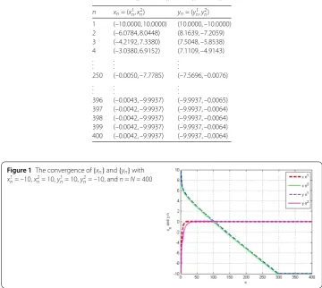
It is clear that the sequences{αn},{μn}satisfy all the conditions of Theorem1, so we
can conclude that the sequences{xn}and{yn}converge strongly to (0, –10) and (–10, 0),
respectively. Table1 shows the values of{xn} and{yn}with x1n= –10,x2n= 10,y1n= 10, y2
[image:20.595.127.456.108.295.2]n= –10, andn=N= 400.
Table 1 The values of{xn}and{yn}withx1n= –10,x2n= 10,y1n= 10,y2n= –10, andn=N= 400
n xn= (x1n,x2n) yn= (y1n,yn2)
1 (–10.0000, 10.0000) (10.0000, –10.0000) 2 (–6.0784, 8.0448) (8.1639, –7.2059) 3 (–4.2192, 7.3380) (7.5048, –5.8538) 4 (–3.0380, 6.9152) (7.1109, –4.9143) .
. .
. . .
. . .
250 (–0.0050, –7.7785) (–7.5696, –0.0076) .
. .
. . .
. . .
396 (–0.0043, –9.9937) (–9.9937, –0.0065) 397 (–0.0042, –9.9937) (–9.9937, –0.0064) 398 (–0.0042, –9.9937) (–9.9937, –0.0064) 399 (–0.0042, –9.9937) (–9.9937, –0.0064) 400 (–0.0042, –9.9937) (–9.9937, –0.0064)
Figure 1The convergence of{xn}and{yn}with
x1
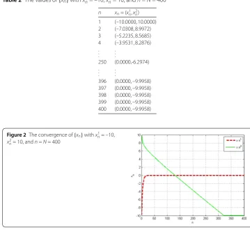
[image:20.595.116.477.411.733.2]Table 2 The values of{xn}withx1
n= –10,xn2= 10, andn=N= 400
n xn= (x1n,x2n)
1 (–10.0000, 10.0000) 2 (–7.0308, 8.9972) 3 (–5.2235, 8.5685) 4 (–3.9531, 8.2876) .
. .
. . .
250 (0.0000,-6.2974) .
. .
. . .
396 (0.0000, –9.9958) 397 (0.0000, –9.9958) 398 (0.0000, –9.9958) 399 (0.0000, –9.9958) 400 (0.0000, –9.9958)
Figure 2The convergence of{xn}withx1n= –10,
x2n= 10, andn=N= 400
Remark1 If we choosef ≡gandxn=ynin Example1, we can rewrite (36) as follows:
xn+1=
4n– 1 7n
xn+
3n+ 1 7n
PC
1 4nf(xn) +
4n– 1 4n
Tnfxn
,
wherePC(x1,x2) = (max{min{x1, 10}, –10},max{min{x2, 10}, –10}) and alsoPC(I–λn∇f) = snI+ (1 –sn)T
f
nandsn=2–λn4(16), whereλn= n 2
8n2+1. From Corollary1, we can conclude that
the sequence{xn}converges strongly to (0, –10). Table2shows the values of{xn} with x1n= –10,x2n= 10, andn=N= 400.
Conclusion
1. Theorem1guarantees the convergence of{xn}and{yn}in Example1. 2. Corollary1guarantees the convergence of{xn}in Remark1.
3. By using the concepts of an intermixed algorithm and gradient-projection algorithm (GPA), we give a new iteration for solving two constrained convex minimization problems.
Acknowledgements
This work is supported by King Mongkut’s Institute of Technology Ladkrabang.
Availability of data and materials Not applicable.
Competing interests
The authors declare that they have no competing interests.
Authors’ contributions
The two authors contributed equally to the writing of this paper. Both authors read and approved the final manuscript.
Publisher’s Note
Springer Nature remains neutral with regard to jurisdictional claims in published maps and institutional affiliations.
Received: 24 April 2019 Accepted: 15 October 2019 References
1. Xu, H.K.: Iterative methods for the split feasibility problem in infinite-dimensional Hilbert spaces. Inverse Probl.26, 105018 (2010)
2. Bretarkas, D.P., Gafin, E.M.: Projection methods for variational inequalities with applications to the traffic assignment problem. Math. Program. Stud.17, 139–159 (1982)
3. Su, M., Xu, H.K.: Remarks on the gradient-projection algorithm. J. Nonlinear Anal. Optim.1, 35–43 (2010) 4. Xu, H.K.: An iterative approach to quadratic optimization. J. Optim. Theory Appl.116, 659–678 (2003) 5. Lions, J.L., Stampacchia, G.: Variational inequalities. Commun. Pure Appl. Math.20, 493–517 (1967)
6. Kangtunyakarn, A.: A new iterative algorithm for the set of fixed-point problems of nonexpansive mappings and the set of equilibrium problem and variational inequalities problem. Abstr. Appl. Anal.2011, Article ID 562689 (2011). https://doi.org/10.1155/2011/562689
7. Ke, Y., Ma, C.: Iterative algorithm of common solutions for a constrained convex minimization problem, a quasi-variational inclusion problem and the fixed point problem of a strictly pseudo-contractive mapping. Fixed Point Theory Appl.2014, 54 (2014)
8. Chahn, Y.-J., Nazeer, W., Naqvi, S.-A., Shin, M.-K.: An implicit viscosity technique of nonexpansive mappings in Hilbert spaces. Int. J. Pure Appl. Math.108(3), 635–650 (2016)
9. Nazeer, W., Munir, M.: Strong convergence of new viscosity rules of nonexpansive mappings. J. Appl. Math.35(5–6), 423–438 (2017)
10. Ceng, L.-C., Ansari, Q.H., Yao, J.-C.: Some iterative methods for finding fixed points and for solving constrained convex minimization problems. Nonlinear Anal.74, 5286–5302 (2011)
11. Ming, T., Liu, L.: General iterative methods for equilibrium and constrained convex minimization problem. J. Optim. Theory Appl.63, 1367–1385 (2014)
12. Yao, Z., Kang, S.M., Li, H.J.: An intermixed algorithm for strict pseudo-contractions in Hilbert spaces. Fixed Point Theory Appl.2015, 206 (2015)
13. Takahashi, W.: Nonlinear Functional Analysis. Yokohama Publishers, Yokohama (2000)
14. Osilike, M.O., Isiogugu, F.O.: Weak and strong convergence theorems for nonspreading-type mappings in Hilbert spaces. Nonlinear Anal.74, 1814–1822 (2011)
15. Opial, Z.: Weak convergence of the sequence of successive approximation of nonexpansive mappings. Bull. Am. Math. Soc.73, 591–597 (1967)
16. Marino, G., Xu, H.-K.: A general method for nonexpansive mappings in Hilbert space. J. Math. Anal. Appl.318, 43–52 (2016)
17. Censor, Y., Elfving, T.: A multiprojection algorithm using Bregman projections in a product space. Numer. Algorithms 8, 221–239 (1994)