BIROn - Birkbeck Institutional Research Online
Cartea, Alvaro and Howison, S. (2006) Option pricing with Lévy-Stable
processes generated by Lévy-Stable Integrated Variance. Working Paper.
Birkbeck, University of London, London, UK.
Downloaded from:
Usage Guidelines:
Please refer to usage guidelines at or alternatively
ISSN 1745-8587
Birkbeck Workin
g
Pa
p
ers in Economics & Finance
School of Economics, Mathematics and Statistics
BWPEF 0602
Option Pricing with Lévy-Stable
Processes Generated by Lévy-Stable
Integrated Variance
Álvaro Cartea
Sam Howison
Option Pricing with L´evy-Stable Processes
Generated by L´evy-Stable Integrated Variance
By ´
Alvaro Cartea
1and Sam Howison
2∗1
Birkbeck College, University of London
2Mathematical Institute, University of Oxford
February 24, 2006
Abstract
In this paper we show how to calculate European-style option prices when
the log-stock price process follows a L´evy-Stable process with index parameter 1≤α≤2 and skewness parameter −1≤β≤1. Key to our result is to model integrated varianceRT
t σs2ds as an increasing L´evy-Stable process with
contin-uous paths.
Keywords: L´evy-Stable processes, stable Paretian hypothesis, stochastic volatil-ity, α-stable processes, option pricing, time-changed Brownian motion.
1
Introduction
Up until the early 1990’s most of the underlying stochastic processes used in the financial literature were based on a combination of Brownian motion and Poisson
∗We are very grateful for comments from Hu McCulloch and seminar participants at the
processes. One of the most fundamental assumptions throughout has been that fi-nancial asset returns are the cumulative outcome of many small events that happen very frequently at a ‘microscopic level’ in time, so that their impact may be regarded as parameterised continuously by time. If these microscopic events are considered sta-tistically independent with finite variance it is straightforward to characterise their limiting cumulative behaviour, as the timestep tends to zero, by invoking the Central Limit Theorem (CLT). Hence, Gaussian-based distributions are a plausible class of models for financial processes.
More generally, dropping the assumption of finite variance, the sum of many iid events always has, after appropriate scaling and shifting, a limiting distribution termed a L´evy-Stable law; this is the generalised version of the Central Limit The-orem, (GCLT), [ST94]; the Gaussian distribution is one example. Based on this fundamental result, it is plausible to generalise the assumption of Gaussian price in-crements by modelling the ‘formation’ of prices in the market by the sum of many stochastic events with a L´evy-Stable limiting distribution.
An important property of L´evy-Stable distributions is that of stability under ad-dition: when two independent copies of a L´evy-Stable random variable are added then, up to scaling and shift, the resulting random variable is again L´evy-Stable with the same shape. This property is very desirable in models used in finance and par-ticularly in portfolio analysis and risk management, see for example Fama [Fam71], Ziemba [Zie74] and the more recent work by Tokat and Schwartz [TS02], Ortobelli et al [OHS02] and Mittnik et al [MRS02]. Only for L´evy-Stable distributed returns do we have the property that linear combinations of different return series, for example portfolios, again have a L´evy-Stable distribution [Fel66].
and prices options using a utility maximisation argument; more recently Carr and Wu [CW03] priced European options when the log-stock price follows a maximally skewed L´evy-Stable process. Cartea and Howison [CH05] also assume that log prices follow a L´evy-Stable process and provide a solution to the pricing problem as a distinguished limit of the L´evy-Stable process.
Finally, based on Mandelbrot and Taylor [Man97], Platen, Hurst and Rachev [HPR99] provide a model to price European options when returns follow a (sym-metric) L´evy-Stable process. In their models the Brownian motion that drives the stochastic shocks to the stock process is subordinated to an intrinsic time process that represents ‘operational time’ on which the market operates. Option pricing can be done within the Black-Scholes framework and one can show that the subordinated Brownian motion is a symmetric L´evy-Stable motion.
The motivation of this paper is as follows. It is well known that if the risk-neutral stock price process follows
ST =Ster(T−t)−
1 2 R
T t σ2sds+
R
T t σsdW
Q
s , (1)
where dWtQ is the increment of the Brownian motion and the volatility is given by a stochastic process σt where σt and WtQ are independent for all 0 ≤ t ≤ T, then
the value of a European vanilla option written on the underlying stock price St with
payoff Π(S, T) is given by
V(S, t) =EQ
"
VBS St, t, K,
1
T −t
Z T
t
σs2ds
1/2
, T
!#
, (2)
where the expected value is with respect to the random variableYt,T =
RT
t σs2dsunder
the risk-neutral measure Q and VBS is the usual Black-Scholes value for a European
option. In general, the distribution or characteristic function of the integrated vari-ance Yt,T is not known, so evaluating (2) is not straightforward, although given the
characteristic function of the integrated variance we can use standard transform meth-ods to evaluate V(S, t) given by equation (2). In this paper we propose a two-factor model where the shocks to the stock process are conditionally Gaussian, ie Brownian motion, and the integrated varianceYt,T follows a L´evy-Stable process, and as a result
The paper is structured as follows. Section 2 presents definitions and properties of L´evy-Stable processes. In particular we show how symmetric L´evy-Stable random variables may be ‘built’ as a combination of two independent L´evy-Stable random variables. Section 3 discusses the path properties required to model integrated vari-ance as a totally skewed to the right L´evy-Stable process. Section 4 describes the dynamics of the stock process under both the physical and risk-neutral measure and shows how option prices are calculated when the stock returns or log-stock process follows a L´evy-Stable process. Finally, section 5 shows numerical results and section 6 concludes.
2
L´
evy-Stable random variables
In this section we show how to obtainany symmetric L´evy-Stable motion as a stochas-tic process whose innovations are the product of two independent L´evy-Stable random variables. The only conditions we require (we will make this precise in Proposition 2) are that one of the independent random variables is symmetric and the other is totally skewed to the right. This is a simple, yet very important, result since we can choose a Gaussian random variable as one of the building blocks together with any other totally skewed random variable to ‘produce’ symmetric L´evy-Stable random variables. Furthermore, choosing a Gaussian random variable as one of the building blocks of a symmetric random variable will be very convenient since we will be able to relate any symmetric L´evy-Stable motion as a conditional Brownian motion, con-ditioned on the other building block, the totally skewed L´evy-Stable random variable which in our case will be the quantity known as integrated variance.
We recall that the log-characteristic function of a L´evy-Stable process Lt is given
by
lnE[eiθLt]
≡Ψt(θ) =
(
−tκα|θ|α{1−iβsign(θ) tan(απ/2)}+imθ for α 6= 1,
−tκ|θ|
1 + 2πiβsign(θ) ln|θ| +imθ for α = 1, (3)
random variableL1 belongs to a L´evy-Stable distribution with parametersα,κ,β,m
we write L1 ∼ Sα(κ, β, m). Bearing in mind the translation invariance with respect
to m and the implicit scaling with respect to κ we define a standard L´evy-Stable motion by Lα,βt ∼ Sα(t1/α, β,0) and the increment by dLα,βt is thought of as having
the distribution Sα(dt1/α, β,0). Finally, we point out that when α < 1 and β =−1
(resp. β = 1) the processLt has support on the negative (resp. positive) line.
It is straightforward to see that for the case 0 < α ≤ 1 the random variable L1
does not have any moments, and for the case 1< α < 2 only the first moment exists (the case α = 2 is Gaussian). Moreover, given the asymptotic behaviour of the tails of the distribution of a L´evy-Stable random variable it can be shown that the Laplace transform E[e−τ L1] of L
1 exists only when its distribution is totally skewed to the
right, that is β = 1, which we state in the following proposition which we use later.
Proposition 1. The Laplace Transform [ST94]. The Laplace transform E[e−τ X]
with τ ≥ 0 of the L´evy-Stable variable X ∼ Sα(κ,1,0) with 0 < α ≤ 2 and scale
parameter κ >0 satisfies
lnE[e−τ X] =
(
−καταsec πα
2 for α6= 1,
2κ
π τlnτ for α= 1.
(4)
The existence of the Laplace transform of a totally skewed to the right L´evy-Stable random variable will enable us to show how to price options as a weighted average of the classical Black-Scholes price when the shocks to the stock process follow a L´evy-Stable process. First we see that any symmetric L´evy-Stable random variable can be represented as the product of a totally skewed with a symmetric L´evy-Stable variable as shown by the following proposition.
Proposition 2. Constructing Symmetric Variables[ST94]. LetX ∼Sα′(κ,0,0),
Y ∼ Sα/α′((cos πα
2α′)
α′
α,1,0), with 0< α < α′ ≤ 2, be independent. Then the random
variable
Z =Y1/α′X ∼Sα(κ,0,0).
3
Stochastic Volatility with L´
evy-Stable Shocks
As motivated in the introduction, the L´evy-Stable hypothesis postulates that the shocks to the stock process must be L´evy-Stable. If we assume that the returns process is given by
dSt
St
=µdt+σtdWt so that ST =eµ(T−t)−
1 2 R
T t σ2sds+
R
T t dWs,
whereµis a constant anddWtthe increment of Brownian motion we could be tempted,
based on Proposition 2, to model volatility by assuming that the integrated variance is given by
Yt,T =
Z T
t
σs2ds=
Z T
t
dLα/s 2,1. (5)
Note thatdLα/t 2,1 is the increment of a positive L´evy-Stable motion so that (5) is an
increasing process. This seems a reasonable choice since
E[eiθ
R
T
t σsdW s] =e−
1
2α/2sec(πα/4)(T−t)|θ|
α
hence the shocks to the process would be symmetric L´evy-Stable, see Proposition 2.
Unfortunately this model for integrated variance is inconsistent since on the left-hand side of (5) we have the integrated variance RT
t σ
2
sds which is, by construction, a
continuous process. However, on the right-hand side of the SDE, we have the nonneg-ative L´evy-Stable motionRT
t dL α/2,1
s which is by construction a purely discontinuous
process. The following subsection discusses a way of constructing a process for the integrated variance that is L´evy-Stable but with continuous paths.
3.1
Sample Path Properties: Modelling Integrated Volatility
In this section we show that it is possible to specify a model for stochastic integrated variance whose finite-dimensional distribution is a totally skewed to the right L´evy-Stable distribution possessing continuous paths. We show that a purely discontinuous process such as the L´evy-Stable motion RT
t dL α/2,1
s can be modified to obtain a
s ∈ R+ in the kernel of RT
t f(s, T)dL α/2,1
s to ‘damp’ the jump process and ‘force’ it
to be continuous in T. In fact we will require that f(s, T) = 0 ass →T so the ‘last’ jumps of the process get smoothed out. (For a general discussion of the path behav-iour of processes of the type RT
t f(s, T)dL α/2,1
s see [ST94].) Since we are interested in
pricing options where the underlying stochastic component is driven by a symmetric L´evy-Stable process we would like to specify a kernelf(s, T) so the finite-dimensional distribution ofRT
t σ
2
sds=
RT
t f(s, T)dL α/2,1
s is totally skewed to the right L´evy-Stable.
As we shall show below, there are many such functions; we denote the class of such functions by F. Below we present a proposition that provides sufficient conditions satisfied by the functions in F.
Proposition 3. Let f(s, T) be a continuously differentiable function and define the
process Xt,T =
RT
t f(s, T)dL α/2,1
s . Then Xt,T is continuous in T.
Proof. Using integration by parts we have that
Z T
t
f(s, T)dLα/s 2,1 = f(s, T)Lα/s 2,1|Tt −
Z T
t
∂f(s, T)
∂s L
α/2,1
s ds
= −f(t, T)Lα/t 2,1 −
Z T
t
∂f(s, T)
∂s L
α/2,1
s ds;
by standard properties of Lα/t 2,1 and since f(s, T) is continuously differentiable, Xt,T
has continuous paths, ie is continuous in T.
Two possible choices for f(s, T) are
f(s, T) = g(T −s) =T −s T ≥ s≥0, (6)
f(s, T) =g(T −s) = 1
γ 1−e
−γ(T−s)n
for T, s≥0 and n≥1, (7)
motion they are driven by a L´evy process, see [Wol82]. Barndorff-Nielsen and Shep-hard [BNS02] were the first to introduce OU-type stochastic volatility models driven by positive L´evy processes. A third choice is
f(s, T) =g(T −s) = ln(T −s+ 1) for T ≥s≥0. (8)
Note that for some purposes it is convenient to require that f(s, T) ≥ 0; all the examples above have this property.
3.2
Illustration
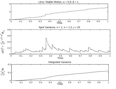
We now illustrate the different building blocks needed to obtain the integrated vari-ance process described above. First we simulate a totally skewed to the right L´evy-Stable motion; then we get the spot variance process, by choosing an appropriate kernel; then we produce the integrated variance process. We focus on kernels of the integrated variance of the form
f(s, T) = g(T −s) = 1
γ 1−e
−γ(T−s)n
.
The solid line in the two bottom graphs of Figure 1 represents the case with n = 1,
t = 0, 0≤ T ≤1 and γ = 25 which would yield a standard OU-type process. In the same figure the dotted lines represent the case n= 1.2, T = 1 and γ = 25. Note that the higher the constant n is the ‘smoother’ is the path of the integrated variance.
4
Model dynamics and option prices
0 0.1 0.2 0.3 0.4 0.5 0.6 0.7 0.8 0.9 1 0
2 4
Time
Lévy−Stable Motion, α = 0.8, β = 1
0 0.1 0.2 0.3 0.4 0.5 0.6 0.7 0.8 0.9 1
0 0.2 0.4 0.6 0.8
Spot Variance, n = 1, n = 1.2, γ = 25
Time
σ
(T)
2 =
∫ 0
T e
−
γ
(T−s)
n dL
s
0 0.1 0.2 0.3 0.4 0.5 0.6 0.7 0.8 0.9 1
0 0.1 0.2
Time
∫ 0
T σ 2 ds s
[image:11.612.125.505.62.353.2]Integrated Variance
Figure 1: Simulated integrated variance with kernelg(T −s) = 25−1 1−e−25(T−s)n
with n= 1, T = 1, solid line, and n= 1.2, T = 1, dotted line.
Given the nature of the model it is obvious that there will not be a unique equiv-alent martingale measure (EMM). In line with most of the L´evy process literature we choose an EMM that is structure preserving since, among other features (see [CT04]), transform methods for pricing are straightforward to implement; this will be discussed at the end of subsection 4.2.
4.1
Modelling returns
distribution we assume that
dSt
St
= µdt+σtdWt (9)
Z T
t
σs2ds = ˆσα/2
Z T
t
g(T −s)dLα/s 2,1, (10)
where dWt denotes the increment of the standard Brownian motion, g(T −s) ∈ F,
ˆ
σ ≥ 0 and µ are constants. In appendix A we show that by modelling integrated variance as in (10) the shocks to the stock process (9) are symmetric L´evy-Stable.
Note that we might also stipulate that our departure point is the risk-neutral dynamics for the stock process and that our model is given as above with µ=r. In this case the risk-neutral dynamics follow
dSt
St
=rdt+σtdWtQ (11)
withRT
t σ
2
sds as in (10). However, we need not specify the risk-neutral dynamics as a
starting point since it is possible to postulate the physical dynamics and then choose an EMM. We discuss this change of measure below for the model that also allows for asymmetric L´evy-Stable shocks and the symmetric case then becomes a particular case.
Before proceeding we remark that the stochastic integral RT
t σsdWs can be seen as
a time-changed Brownian motion [KS02]. In this case the integrated varianceRT
t σ
2
sds
represents the time-change and it is straightforward to show that
Z T
t
σsdWs d
=WTˆt,T
where ˆTt,T =
RT
t σ
2
sds.
4.2
Modelling Log-Stock Prices
In stochastic volatility models one way to introduce skewness in the log-stock process is to correlate the random shocks of the volatility process to the shocks of the stock process. It is typical in the literature to assume that the Brownian motion of the stock process, say dWt, is correlated with the Brownian motion of the volatility
process, say dZt. Thus E[dWtdZt] = ρdt and we can write ˜Zt = ρWt+
p
1−ρ2Z
t,
where ˜Zt is independent of Wt. The correlation parameter ρ is also known in the
literature as the leverage effect and empirical studies suggest thatρ <0 [FPS00]. In our case we may also include a leverage effect via a parameter ℓ to produce skewness in the stock returns. However, the notion of ‘correlation’ does not apply in our case because for L´evy-Stable random variables, as given that moments of second and higher order do not exist, nor do correlations.
Hence to allow for asymmetric L´evy-Stable shocks, under the physical measure we assume that
ln(ST/St) = µ(T −t) +
Z T
t
σsdWs+ℓσ˜α
Z T
t
dL˜α,s −1 (12)
Z T
t
σ2sds = ˆσα/2
Z T
t
g(T −s)dLα/s 2,1. (13)
Here dWt denotes the increment of the standard Brownian motion independent of
both dL˜α,t −1 and dLtα/2,1 and we note that dL˜α,t −1 is totally skewed to the left and that α <2, ie the stability index α is not restricted to be less than unity. Moreover,
µ, ˜σ ≥0, ˆσ ≥ 0 are constants, g(T −s) ∈ F and the leverage parameter ℓ ≥ 0.1 In
appendix B we show that the shocks to the price process are asymmetric L´evy-Stable.
Before proceeding we discuss the connection of the dynamics of the stock price un-der the physical measureP and the risk-neutral measure Q. Recall that a probability
1Note that here we model log-stock prices since wecannot include a leverage effect in equation
(9) in the form
dSt
St =
µdt+σtdWt+ℓσ˜αdL˜α,t −1 (14)
Z T
t
σ2sds = σˆα/2
Z T
t
g(T−s)dLα/s 2,1,
because the solution to the SDE with leverage (14) will deliver a stock processStthat allows negative prices due to the jumps of the increments of the L´evy-Stable motiondL˜α,−1
measure Q is called an EMM if it is equivalent to the physical probabilityP and the discounted price process is a martingale. It is straightforward to see that in the model proposed here the set of EEMs is not unique, hence we must motivate the choice of a particular EMM. Based on Theorem 3.1 in [NV03] we choose a structure-preserving measure where the risk-neutral dynamics of the model (12) and (13) follows
ln(ST/St) = r(T −t)−
Z T
t
σs2ds+ 1
2(T −t)ℓ
ασα ℓ sec
πα
2 +
Z T
t
σsdWsQ+ℓσ˜α
Z T
t
dL˜α,s −1.
Note that if ℓ = 0 we obtain the risk-neutral dynamics for the case when the returns or log-stock process follows a symmetric L´evy-Stable process underP.
4.3
Option Pricing with L´
evy-Stable Volatility
The preceding sections were devoted to finding a suitable model for stochastic volatil-ity that would enable us to model the unconditional returns process or log-stock process as a L´evy-Stable process. Moreover, as motivated in the introduction by equations (1) and (2), it is straightforward to see that if we assume the dynamics given by (12) and (13) the price of a vanilla option is given by the iterated expecta-tions
V(S, t) =EQL˜α,−1
t
"
EQσt
"
EQ
"
VBS Steℓ
R
T
t dL˜s, t, K,
1
T −t
Z T
t
σs2ds
1/2
, T
!#
˜
Lα,t −1, σt|L˜α,t −1
##
,(15)
whereQis the risk-neutral measure andVBS is the Black-Scholes value for a European
option.
Remark 1. Note that if we let g(T −s) = 0 then the model reduces to
ln(ST/St) = µ(T −t) +ℓσ˜α
Z T
t
dL˜α,s −1,
which is the Finite Moment Log-Stable (FMLS) model of [CW03].
Proposition 4. It is possible to extend the results above to price European call and
Proof. Using put-call inversion [McC96], we have by no-arbitrage that European call
and put options are related by
C(S, t;K, T, α, β) =SKP(S−1, t;K−1, T, α,−β).
Note that using put-call inversion allows us to obtain put prices when the log-stock price follows a positively skewed L´evy-Stable process, based on call prices where the underlying log-stock price follows a negatively skewed L´evy-Stable process. Further-more, put-call parity allows us to obtain call prices when the skewness parameter
−1≤β ≤0.
As an example, we can use the approach above to derive closed-form solutions for option prices when the random shocks to the price process are distributed according to a Cauchy L´evy-Stable process, α= 1 and β= 0.
Remark 2. Closed-form Solution when Returns follow a Cauchy Process.
By letting α = 1 and ℓ = 0 in (12) and (13) we have that option prices, under the risk-adjusted measure Q, are given by
V(S, t) =
RT
t g(T −s)
1/2ds
(T −t)√2π
Z ∞
0
VBS(St, t, K, Y
1/2
t,T, T)
1
y3/2e
−
R
T
t g(T−s)1/2ds T−t
2
/2y
dy,
where Yt,T = T1−t
RT
t σ
2
sds.
To see this, first we note that the combination of a Gaussian, the Brownian motion in (12), and L´evy-SmirnovS1/2(κ,1,0), the process followed by the integrated variance
in (13), random variables results in a Cauchy random variable S1(κ,0,0). This can
be seen by calculating the convolution of their respective pdf’s. Now, recall that the pdf for a L´evy-Smirnov random variableS1/2(κ,1,0) is given by (κ/2π)1/2x−3/2e−κ/2x
with support (0,∞); hence in our case the distribution of the average integrated variance is given by
Y ≡ 1 T −t
Z T
t
g(T −s)dLα/2,1
s ∼S1/2
1 (T −t)2
Z T
t
g(T −s)1/2ds
2
,1,0
!
thus the value of the option is
V(S, t) =
RT
t g(T −s)1/2ds
(T −t)√2π
Z ∞
0
VBS(St, K, Y
1/2
t,T, T)
1
y3/2e
−
R
T
t g(T−s)1/2ds T−t
2
/2y
dy.
5
Numerical illustration: L´
evy-Stable Option Prices
In this section we show how vanilla option prices are calculated according to the above derivations. One route is to calculate the expected value of the Black-Scholes formula weighted by the stochastic volatility component and the leverage effect. Another route to price vanilla options for stock prices that follow a geometric L´evy-Stable processes is to compute the option value as an integral in Fourier space, using Complex Fourier Transform techniques [Lew01], [CM99].
We use the Black-Scholes model as a benchmark to compare the option prices obtained when the returns follow a L´evy-Stable process. Our results are consistent with the findings in [HW87] where the Black-Scholes model underprices in- and out-of-the-money call option prices and overprices at-the-money options.
5.1
Option Prices for Symmetric L´
evy-Stable log-Stock Prices
In this subsection we obtain option prices and implied volatilities when the log-stock prices follow symmetric L´evy-Stable process. Recall that, under the risk-neutral measure Q, the stock price and variance process are given by
ST = Ster(T−t)−
1 2 R
T t σ2sds+
R
T t σsdW
Q s ,
Z T
t
σs2ds = ˆσα/2
Z T
t
g(T −s)dLα/s 2,1.
The first step we take is to calculate the characteristic function of the process
Zt,T =−
1 2
Z T
t
σs2ds+
Z T
t
Proposition 5. The characteristic function of Zt,T is given by
EQ[eiξZt,T] =e−21σαLS(iξ+ξ2) α/2R
T
t g(T−s)2/αds, (16)
where ξ =ξr+iξi and −1≤ξi ≤0 andσLS ≥0 (see (20) in appendix A). Moreover,
the characteristic function is analytic in the strip −1< ξi <0.
Proof. The characteristic function is given by
EQeiξZt,T = EQ
h
e−12iξ R
T t σ2sds+iξ
R
T t σsdWs
i
= EQ
h
e−12iξ R
T
t σ2sds−12ξ2 R
T t σ2sds
i
= EQhe−12(iξ+ξ2) R
T
t g(T−s)dL α/2,1
s i
= e−12σαLS(iξ+ξ2) α/2R
T
t g(T−s)2/αds.
The last step is possible since the expected value exists if ξ is restricted so that
ξ2
r −ξi2+ξi ≥ 0, by consideration of the penultimate line. The region where this is
true contains the strip−1≤ξi ≤0. Finally, it is straightforward to observe that the
characterisitc function is analytic in this strip.
To price call options we proceed as above and use the following expression:
C(x, t) =ext − 1
2πe
−r(T−t)K
iξi+∞
Z
iξi−∞
e−iξxt K
iξ
ξ2−iξe
(T−t)Ψ(−ξ)dξ (17)
where xt = lnSt, 0 < ξi < 1, and Ψ(ξ) is the characteristic function of the process
lnST.
5.1.1 Numerics for Symmetric L´evy-Stable log-Stock Prices
relevant parameters of the two models. In fact, the only parameter that we must care-fully examine is the scaling parameter of the L´evy-Stable process; we opt for one that can be related to the standard deviation used when the classical Black-Scholes model is used. One approach is to proceed as in [HPR99] and match a given percentile of the Normal and a symmetric L´evy-Stable distribution. For example, if we want to match the first and third quartile of a Brownian motion with standard deviation σ = 0.20 to a symmetric L´evy-Stable motion κdLα,0 with characteristic exponent α = 1.7, we
would require the scaling parameter κ = 0.1401. We have chosen these parameters so that for options with 3 months to expiry these quartiles match. Moreover, in the examples below, we use the kernel g(T−s) = 1
25 1−e
−25(T−s)
where for illustrative purposes we have assumed mean-reversion over a two week period, ie γ = 25.
Figure 2 shows the difference between European call options when the stock re-turns are distributed according to a symmetric L´evy-Stable motion with α = 1.7 and when returns follow a Brownian motion with annual volatility σBS = 0.20. The
figure shows that for out-of-the-money call options the L´evy-Stable call prices are higher than the Black-Scholes and for at-the-money options Black-Scholes delivers higher prices. These results are a direct consequence of the heavier tails under the L´evy-Stable case.
5.2
Option Prices for Asymmetric L´
evy-Stable log-Stock Prices
In this subsection we obtain option prices and implied volatilities when there is a negative leverage effect, ie log-stock prices follow an asymmetric L´evy-Stable process. Recall that, under the risk-neutral measure Q, the stock price and variance process are given by
ST = Ster(T−t)−
1 2 R
T
t σs2ds+12(T−t)ℓασℓαsecπα2 + R
T t σsdW
Q s +ℓσ˜α
R
T t dL˜
α,−1
s ,
Z T
t
σs2ds = ˆσα/2
Z T
t
g(T −s)dLα/s 2,1.
We proceed as above and calculate the characteristic function of the process
Zt,Tℓ =−1 2
Z T
t
σs2ds+
Z T
t
σsdWs+ℓσ˜α
Z T
t
0 20 40 60 80 100 120 140 160 180 200 −1.4 −1.2 −1 −0.8 −0.6 −0.4 −0.2 0 0.2 0.4 Strike Price
£ 1 month3 months
[image:19.612.141.470.64.257.2] [image:19.612.94.455.499.700.2]6 months
Figure 2: Difference between L´evy-Stable and Black-Scholes call option prices for dif-ferent expiry dates: one, three and six months. In the Black-Scholes annual volatility is σBS = 20%.
Proposition 6. The characteristic function of Zℓ
t,T is given by
EQ[eZℓt,T] =e−
1 2
σα
LS(iξ+ξ2) α/2R
T
t g(T−s)2/αds+(T−t)(iξℓ)ασℓαsecπα2
, (18)
where −1≤ξi ≤0, ξ =ξr+iξr. Moreover, the characteristic function is analytic in
the strip −1< ξi <0.
Proof. The proof is very similar to the one above. It suffices to note that for ξi ≤0
E
Qheiξ
R
T t dL˜
α,−1 s i ≤ E Qh e iξ R T t dL˜
α,−1 s i
= EQhe−ξi
R
T t dL˜
α,−1
s i
< ∞.
Moreover, for ξi <0 we have that EQ
h
eiξ
R
T t dL˜
α,−1
s
i
is analytic, ie
d dξE
Qheiξ
R
T t dL˜
α,−1 s i = E Q i Z T t
dL˜α,s −1eiξ
R
T t dL˜
α,−1 s
0 20 40 60 80 100 120 140 160 180 200 0
0.5 1 1.5 2 2.5 3 3.5 4
Strike Price
Implied Volatility (%)
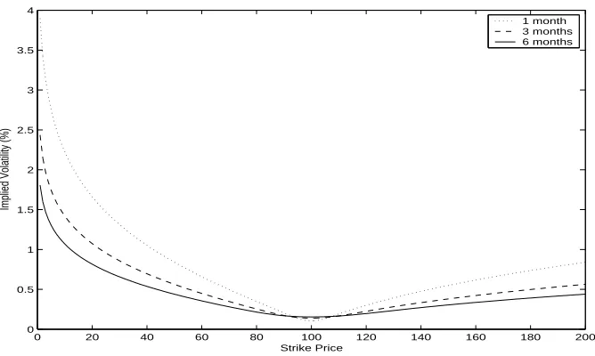
[image:20.612.139.473.58.258.2]1 month 3 months 6 months
Figure 3: Black-Scholes implied volatility for the L´evy-Stable call option prices when returns follow a symmetric L´evy-Stable motion withα = 1.7,β = 0 and three expiry dates: one, three and six months.
Putting these results together with the results from Proposition 5 we get the desired result. Note that the requirement is −1< ξi <0 because dL˜α,t −1 is totally skewed to
the left, therefore we need −ξi >0.
We use the same g(T−s) as above and include a leverage parameterℓ = 1 so that returns follow a negatively skewed process withβ(t, T) =−0.5 when there is 3 months to expiry. Figure 4 shows the difference between L´evy-Stable and Black-Scholes call option prices for different expiry dates. In the Black-Scholes case annual volatility is σBS = 0.20 and in the asymmetric L´evy-Stable case with scaling coefficient σℓ =
0 20 40 60 80 100 120 140 160 180 200 −0.4
−0.2 0 0.2 0.4 0.6 0.8 1
Strike Price
£
[image:21.612.138.473.71.269.2] [image:21.612.138.471.391.591.2]1 month 3 months 6 months
Figure 4: Difference between L´evy-Stable and Black-Scholes call option prices for dif-ferent expiry dates: one, three and six months. In the Black-Scholes annual volatility is σBS = 0.20 and in the asymmetric L´evy-Stable case the scaling parameters are
σLS = 0.7673 and σℓ = 0.1401.
0 20 40 60 80 100 120 140 160 180 200 0
0.5 1 1.5 2 2.5 3 3.5 4
Strike Price
Implied Volatility (%)
1 month 3 months 6 months
Figure 5: Black-Scholes implied volatility for the L´evy-Stable call option prices when returns follow a symmetric L´evy-Stable motion with α = 1.7, σLS = 0.7673 and
6
Conclusion
A
Appendix A
Here we show that if the stock process, as assumed above in section 4.1, follows
dSt
St
= µdt+σtdWt
Z T
t
σs2ds = ˆσα/2
Z T
t
g(T −s)dLα/s 2,1,
where dWt denotes the increment of the standard Brownian motion, g(T −s)∈F, ˆσ
and µ are constants, it is straightforward to show that the shocks to the process are symmetric L´evy-Stable.
First note that the stochastic component of the log-stock process is given by
Ut,T =
Z T
t
σsdWs. (19)
and for convenience choose2
ˆ
σ= 2
1 2cos
πα
4
2/α
σ2LS. (20)
Now we calculate the characteristic function of the random process Ut,T. We have
E[eiθUt,T] =E[eiθ
R
T
t σsdWs],
and conditioning on the path ofσs for t≤s≤T and using iterated expectations we
get
E[eiθUt,T] =Ehe−12θ2
R
T t σ2sds
i
.
Now, given that RT
t σ2sds =
RT
t g(T −s)dL α/2,1
s and using Proposition 1 we write
E[eiθUt,T] = Ehe−12θ2
R
T
t g(T−s)dL α/2,1
s i
= e−12σαLS
R
T
t g(T−s)2/αds|θ|α.
This is clearly the characteristic function of a symmetric L´evy-Stable process with index α.
2We chose ˆσin this way just for convenience in the calculations since it does not have any effect
B
Appendix B
Suppose that the stock process, as assumed above in section 4.2, follows
ln(ST/St) = µ(T −t) +
Z T
t
σsdWs+ℓσ˜α
Z T
t
dL˜α,s −1
Z T
t
σ2sds = ˆσα/2
Z T
t
g(T −s)dLα/s 2,1,
under P where dWt denotes the increment of the standard Brownian motion
inde-pendent of both dL˜α,t −1 and dLα/t 2,1. Then it is straightforward to verify that the shocks to the above log-stock process under the measureP are those of a L´evy-Stable process with negative skewness β ∈(−1,0]. Let G(t, T) =RT
t g(T −s)α/2ds and, for
simplicity in the calculations, assume that ˆσ is given by (20) and
˜
σ= 1
21/ασℓ. (21)
Now consider the process
Ut,Tℓ =
Z T
t
σsdWs+ℓ
Z T
t
dL˜α,s −1.
The characteristic function of Uℓ
t,T is given by
E
h
eiθUt,Tℓ
i
= Eheiθ(
R
T
t σsdWs+ℓσ˜α
R
T t dL˜
α,−1
s )i
= e−12G(T,t)σLSα |θ|αE
h
eiθℓ˜σα
R
T t dL˜
α,−1
s i
= e−12G(t,T)σα
LS|θ|αe−12(T−t)ℓασαℓ|θ|α{1+isign(θ) tan(πα/2)}
= e−
1
2(G(t,T)σαLS+(T−t)ℓασαℓ)|θ| α
1− −(T−t)ℓασαℓ
G(t,T)σαLS+(T−t)ℓασαℓisign(θ) tan(πα/2)
.
This is obviously the characteristic function of a skewed L´evy-Stable process with skewness parameter
β(t, T) = −(T −t)ℓ
ασα ℓ
G(t, T)σα
LS + (T −t)ℓασℓα
∈(−1,0].
Moreover, when ℓ= 0 we obtain β = 0 andβ → −1 asℓ→ ∞ .
Note that the integrated variance does not have a finite first moment since α/2<
1. However, in the case of the leverage effect RT
t dL˜α,s −1 its first moment exists, ie
E[RT
References
[BNS02] O.E. Barndorff-Nielsen and N. Shephard. Financial volatility, L´evy processes and power variation. Unpublished book, Nuffield College, June 2002.
[CH05] A. Cartea and S. Howison. Distinguished limits of L´evy-Stable processes,´ and applications to option pricing. Working Paper Mathematical Institute, University of Oxford, December 2005.
[CLM97] J.Y. Campbell, A.W. Lo, and A.C. MacKinlay. The Econometrics of Fi-nancial Markets. Princeton, 1st edition, 1997.
[CM99] P. Carr and D. Madan. Option valuation using the fast fourier transform.
Journal of Computational Finance, 2:61–73, 1999.
[CT04] R. Cont and P. Tankov. Financial Modelling With Jump Processes. Chap-man and Hall, 2004.
[CW03] P. Carr and L. Wu. The finite moment logstable process and option pricing.
The Journal of Finance, LVIII(2):753–777, April 2003.
[Fam71] E. Fama. Risk, Return and Equilibrium. The Journal of Political Economy, pages 30–55, 1971.
[Fel66] W. Feller. An Introduction to Probability Theory and its Applications, vol-ume II. Wiley, 1966.
[FPS00] J.P. Fouque, G. Papanicolaou, and K.R. Sircar. Derivatives in Financial Markets with Stochastic Volatility. Cambridge, 1st edition, 2000.
[HPR99] S.R. Hurst, E. Platen, and S.T. Rachev. Option pricing for a logstable asset price model. Mathematical and Computer Modelling, 29:105–119, 1999.
[KL76] A. Kraus and R.H. Litzenberger. Skewness preference and the valuation of risk assets. The Journal of Finance, 31(4):1085–1100, September 1976.
[KS02] J. Kallsen and A. N. Shiryaev. Time change representation of stochastic integrals. Theory of Probability and Its Applications, 46(3):522–528, 2002.
[Lew01] A. Lewis. A simple option formula for general jump-diffusion and other exponential L´evy processes. Working Paper, September 2001.
[Man97] B. Mandelbrot.Fractals and Scaling in Finance. Springer, 1st edition, 1997.
[McC96] J.H. McCulloch. Statistical Methods in Finance, volume 14, chapter Finan-cial Applications of Stable Distributions, pages 393–425. Elsevier Science, 1996.
[MRS02] S. Mittnik, S. Rachev, and E. Schwartz. Value-at-risk and asset allocation with stable return distributions. Allgemeines Statistisches Archiv, pages 53–68, 2002.
[NV03] E. Nicolato and M. Venardos. Option pricing in stochastic volatility mod-els of the ornstein-uhlenbeck type. Mathematical Finance, 13(4):445–466, October 2003.
[OHS02] S. Ortobelli, I. Huber, and E. Schwartz. Portfolio selection with stable distributed returns. Mathematical Methods of Operations Research, 2002.
[ST94] G. Samorodnitsky and M. Taqqu. Stable Non-Gaussian Random Processes, Stochastic Models with Infinite Variance. Stochastic Modelling. Chapman Hall, 1st edition, 1994.
[TS02] Y. Tokat and E. Schwartz. The impact of fat tailed returns on asset allo-cation. Mathematical Methods of Operations Research, 2002.
[Wol82] S.J. Wolfe. On a continuous analogue of the stochastic difference equation