DETECTION ENVIRONMENT FORMATION METHOD FOR ANOMALY DETECTION SYSTEMS

(1)

Journal of Theoretical and Applied Information Technology 31st_{August 2019. Vol.97. No 16}

ISSN: 1992-8645 www.jatit.org E-ISSN: 1817-3195

4453

THE IMPLEMENTATION OF THE OPTIMAL RULE BASES

GENERATED BY HYBRID FUZZY C-MEAN AND PARTICLE

SWARM OPTIMIZATION

1_{ACHMAD EFENDI,} 2_{SAMINGUN HANDOYO,}3_{ARI P.S. PRASOJO,} 4 _MARJI

1,2_{Department of Statistics, Universitas Brawijaya Malang, Indonesia}

3_{Indonesian Institute of Science (LIPI), Jl. Gatot Subroto 10 Jakarta 12710, Indonesia} 4_{Department of Informatics Engineering, Universitas Brawijaya Malang, Indonesia}

E-mail: 1_{[email protected],}2_{[email protected],}3_{[email protected],}4_{[email protected]}

ABSTRACT

The aims of the paper are to generate fuzzy rule bases that be optimized through fuzzy c-means (FCM) and particle swarm optmization (PSO), and to develope the fuzzy inference systems (FIS) that have the system inputs are combination between the number of linguistic values and the number of assumed lags influence to the system output. The outputs of FCM including are the cluster centers and partition matrix. The number of rules in the fuzzy rule bases formed by FCM is the same as the number of clusters. The cluster centers are used as the center parameters of the Gaussian membership function (MF), while the elements of partition matrix are used to determine the optimal spread parameters of Gaussian's MF through PSO algorithm. The identification of system input variables is done using plot partial autocorrelation function (PACF). The formation of a tentative model based on significant PACF values to construct the input-output pairs matrix which is subsequently grouped by using FCM. The implementation of FIS uses the exchange rate of USD to IRD dataset that is obtained four significant PACF values on lags of k = 1, 5, 8, and 10 which are subsequently used as input variables. Based on the four input variables, systems with 2 inputs, 3 inputs, and 4 inputs combined with the number of clusters of n = 3, 5, and 7 formed 21 systems. Based on the values of both MAPE and R2_{that is obtained the result that in training data if the number of input} variables and number of clusters are increased then the system has the better performance, but in the testing data, the system performance decresed when the number of input variables and the number of clusters.are increased. The best performing system is the system with 2 inputs and 5 clusters.

Keywords: Exchange rate, Fuzzy C-Means, Generating rule bases, Particle Swarm Optimization

1. INTRODUCTION

Knowledge of events that will occur in the future is one factor to win the competition in the global era. There are two types of predictive models, namely classification models and forecasting models. The classification model aims to predict a class of an object based on several features or characteristics as system inputs, while the forecasting model aims to predict the value of a variable in the future based on patterns that existed in the past as system inputs. The desire to produce a system that can classify an object or can forecast future value accurately has led to a hybrid method. Widodo and Handoyo [1], and also Nugroho et al. [2].had done the hybrid methods between Logistic

(2)

4454 methods utilize the advantage of ARIMA that is able to model the black-box in the form of a linear system well and the superiority of machine learning which capable in modeling of a complex nonlinear system well. The hybrid method assumes that the data pattern is composed both linear and non-linear components, the linear pattern was handled by ARIMA and the nonlinear pattern was handled by machine learning method.

The ANN-FIS hybrid model uses the gradient descent optimization principle to generate optimal Membershib Function (MF) parameters that are used on a fuzzy rule base [5, 6, 7]. If given the optimal MF parameters then the fuzzy rule bases used in the inference engine is also optimal. It can lead the system produce output accurately. In the ANN-FIS hybrid method, the dominant role lies in the FIS implementation assuming that the fuzzy rule bases (frb) used on the FIS is the optimal frb, but there is absolutely no guarantee. The number of input variables that influnce the system output have importannt role. If the system is a causality system which the predictor variables are known with certainty then the ANN-FIS hybrid model is feasible to apply, in the other hand, the predictor variables must be identified by using the identification method in time series analyses that usually uses the partial autocorrelation plot [10,11]. Commonly, the frb is given by an expert or the frb generated by using the input-output data pairs. There are some methods for generating the frb including Wang and Mandel [12], Nozaki et al [13] and Arif et al. [14]. Wang and Mendel are pioneer in generating frb by an empirical data and their method popularly was called the table lookup schema [12]. The simpler method called heuristic approach was proposed by Nozaki et al. [13], while Arif et al. [14] used an association rule mining technique for generating frb. The methods of generating the frb above will result in a large number of rules and even the heuristic approach will be an increase in the number of rules exponentially if the number of input variables or the number of linguistic values increase.

The generating frb that produces a small number of rules can use the clustering methods such as the fuzzy subtractive clustering (FSC) [15]. One of the outputs of the clustering method is the cluster center which will be utilized as the center parameter of MF. In practice, the application of FSC has the constrain in determining of cluster number which depend on the radius parameter. As the other choice in generating frb by clustering

method applied the fuzzy c-means where the custer number was given as the input argument [16,17]. The uutilization of cluster center as the center of membership function (MF) still leaves a problem because there is the other parameter in MF.called the spread parameter. The degree of membership of an observation in Gaussian MF depends on the values of both center and spread parameter. Beside the cluster center, the fuzzy c-means also has the additional output called the partition matrix that has the elements as a degree of membership of each observation at its cluster center. To calculate the spread parameters corresponding to the elements of the partition matrix is a non-linear optimization problem. Handoyo and Marji [18] use the ordinary least square optimization to handle the optimization in FIS. There is also a very popular optimization method known as Particle Swarm Optimization (PSO) [19,20]. Handoyo et al [21] had implemented PSO for parameter estimation of ARMA model with high accuracy result.

Based on the above exposure to produce a system capable for predicting accurately, the paper proposed FIS-Takagi Sugeno hybrid method based on both FCM and PSO with the initialization of system input variables using the plot of PACF values on various lags. The FCM method is used to generate the fuzzy rule bases and the PSO method for calculating the optimal spread parameters based on the partition matrix of the FCM output. In this study, we investigate the effect of the number of input variables and the number of clusters on the performance of the system based on two performance indicators that are MAPE and R2_{, and} also will be selected the best performing system.

2. LITERATURE REVIEW

(3)

4455 as a tool of order identification of the autoregressiveve process.

2.1 Partial Autocorrelation Function (PACF)

PACF is an autocorrelation measure considering the lag effect. According to Cryer and Chan [10], PACF on the k-th lag is the correlation between and after the omitted influence of the variables and . The PACF is estimated by the sample partial autocorrelation function (SPACF), denoted as and formulated as follows:

, and

(1)

is the estimator of the autocorrelation coefficient, which is formulated by equation (2):

(2) For the purpose of testing the significance of SPACF values, the interval as the limits of the 95% confidence interval of .

2.2.The Fuzzy Inference System (FIS)

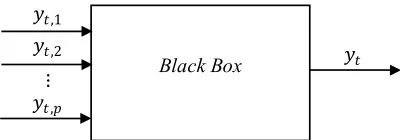
The mechanism of a system can be explained by using an equation called a mathematical model. Complex systems have complex mathematical models. The complexity in question is to contain complex structures, i.e. non-linear elements, randomness, and others. According to Chen and Pham [20], the basic concept of modelling can be illustrated by the unknown relationship of input-output pairs. In general, systems that connect input-output are known as black-box. The Figure 1 is an example of a causal relationship for multiple input and single output cases.

Black Box

𝑦𝑡,1

𝑦_𝑡,2

⋮ 𝑦_𝑡,𝑝

[image:3.612.94.294.569.639.2]

𝑦_𝑡

Figure 1. The system model is considered as black box

The black-box in Figure 1 acts as a connection

between input and output

. In the application, the black-box can be approached by a model including the fuzzy inference system (FIS). FIS consists of 4 basic

components, namely: fuzzy rule base, fuzzification, inference engine, and defuzzification [22].

The fuzzy rule bases take the form of some "IF ... THEN ..." implication, the part following the IF is called the antecedence, and the part following the THEN is consequence. Fuzzification is a process of input mapping in the form of a crisp value into a linguistic value and a degree of membership. The inference engine is an inference process to generate an output of an input pair by following the rules defined in the fuzzy rule bases. Defuzzification is the process of converting the output of an inference engine in the form of a fuzzy set into a system output in the form of a crisp value [23].

2.3.FIS Model of Takagi-Sugeno First Order

Considered symbol L is the number of rules on the fuzzy rule bases for l = 1,2, ..., L that shows the rule indexes, and for k = 1,2, ..., p that indicates the input indexes. According to Palit and Popovic [24], the inference process in Fuzzy Takagi-Sugeno model is divided into 2 stages. The first one is the calculation of a degree of activation (fire strength) for each rule on a fuzzy rule basis. The second stage is the calculation of the system output which is a cirsp value calculated by using the average method. In general, the form of a fuzzy rule in the first order of the Fuzzy Takagi-Sugeno model is as follows:

r (3)

where is the value of the k-th input variable, is the local output (output produced by the l-th rule), is the consequent parameter in rule l, and is the fuzzy set of k-input variables for the l-th rule represented by a membership function . In this research is used the Gaussian membership function (gaussmf) expressed in (4) as follows:

(4) where is the center and is the pread parameters of gaussmf corresponding to the antecedents part of the l-th rule. The fire strength of the l-th rule of the t-th observation is calculated by the multiplication operator as follows:

(4)

4456 where p is the number of input variables. The fire strength is normalized by using equation (6) as follows:

(6) The output of the system in the form of a crisp value is the prediction value of the t-th observation that is calculated by the formula:

(7) The equation (7) is used to the defuzzification process by the weighted average method. The weights that used in the Takagi-Sugeno model are normalized fire strength . The consequent part is a linear equation. Parameters of linear equations in consequent part are estimated by using ordinary least squares (OLS) method.

2.4. The Fuzzy Rules Bases Generated with the Fuzzy C-Mean Clustering

The clustering method can be interpreted as an attempt to group individuals or to group records into multiple clusters based on similarity of properties or features so the objects in one cluster will be relatively homogeneous and the interclass objects are relatively heterogeneous. The main purpose of clustering is to form optimal grouping patterns according to the nature of the data. Therefore the clustering method can be used to generate a rule bases with a number of rules equal to the number of clusters. The basic concept of the clustering method is to group the input-output pair into a cluster and to generate a one rule of each cluster [25].

The Fuzzy C-Means (FCM) clustering is one of the algorithm used for clustering purposes. The clustering process in FCM is to find the partition matrix U and center cluster C by iteration. The elements of matrix U are the degree of input-output pairs membership in each cluster, the general form of the matrix U is:

(8) where q denotes the number of cluster, is the maximum lag considered in the analysis and n denotes the size of the observation. The notation shows the membership degree

of the t-th observation

on the h-th cluster , so the matrix U has the order . The general form of the cluster central C matrix is:

(9) where p is the number of inputs, so the order of C is

and respectively indicate the value of the k-th input variable's center value and the output center value of the output variable on h-th cluster.

The h-th line .of the matrix U and elements of the matrix C in the study is used to estimate the parameter spread of gaussmf by fitting curves. According to Palit and Popovic [24], the fitting is between y(t, k) and the degree of input-output pair membership in the cluster . The fittings are the same as in the regression method, ie approaching the observation point by a curve that can minimize the distance between each observation point and the curve. The principle is to minimize the sum square errors (SSE). The objective function of SSE is formulated by the equation (10).

(10)

Where,

:

the spread parameter of the gaussmf for _{the k-input variable}

:

the center value of the k-th input variable _{in the h-th cluster as the central parameter}

of gaussmf

:

the _{observation on the h-th cl cluster}membership degree of t-th

:

the value of k-th input variable at time t-th _observation

:

number of clusters

:

Number of input variables

Through equation (10) we will estimate a optimal spread parameter written with:

(11) The function in equation (10) is a non-linear function. One of the optimization technique that can be applied to solve equation (11) is Particle Swarm Optimization [20].

(5)

4457 Particle Swarm Optimization (PSO) is part of evolutionary computing techniques. According to Hung [26], PSO is a population-based stochastic optimization technique. The working principle of PSO is inspired by the social behavior of animals such as fish, birds and insects. The social behavior referred to in this context is the behavior of individuals based on their intelligence and the influence of their collective herds. Thus if an individual (eg bird on a bird flock) finds the shortest path to the source of food, then the other individual will follow that path even though the position between individuals is far apart [27].

PSO is able to solve optimization problems in complex multidimensional spaces. Each individual on the PSO has 2 important characteristics that are a position and a speed. Each individual will move in a certain space and remember the best position which ever be passed. The best position is the position where there is a food source or a minimum or maximum objective function value. Individuals will convey the best position information to other individuals, and the other individuals will adjust the speed and position according to the information received.

One type of PSO model is the standard contemporary type. According to Parsopoulos and Vrahatis [28], the contemporary standard PSO is considered a generalization of the PSO model and can work dynamically to achieve convergence. The standard contemporary PSO model is presented in equation (12) as follows:

,

for

(11) where,

: the speed of the i-th individual in the it-th iteration

: the position of the i-th individual on the it-th iteration

: constriction factor

: weighting (PSO parameter)

: a uniformly distributed random number [0,1]

: the best position ever passed by the i-th individual

: best position (global optimum) : iteration counter

: population size (number of individuals) while the constriction factor is calculated by:

, with

and (13)

2.5.

Precision Indicators of Forecasting

Method

The accuracy of forecasting methods is fundamental in forecasting business. The purpose of assessing the accuracy of forecasting methods is to select the correct forecasting method. Accuracy refers to the goodness or suitability of a model. One type of accuracy indicator used to measure the accuracy of a forecasting method is Mean Absolute Percentage Error (MAPE). According to Makridakis et al [29], MAPE is included in relative accuracy indicator. Another standard measure of precision is the coefficient of determination having a range of values between 0 and 1 [30]. The formula both MAPE and are given as follows:

and,

where is the actual output and is prediction value (the system output).

The calculation of is actually the quadratic correlation between the actual value and the predicted value. Actual values and prediction values are analogous to two variables in the simple linear regression. Regardless of the relation of causality, can be calculated by the square of the correlation between the two variables. If the predicted value is close to the actual value then both will form a strong linear relationship. So, in this case, is defined as the size of the match between the actual value and the predicted value.

3. RESEARCH METHOD

(6)

4458 tentative model will be modeled with Fuzzy Takagi-Sugeno model based on FCM-PSO, and finally select the best model based on MAPE and R2_{indicators. The method of analysis is expressed} in 7 steps as follows:

1. Divide dataset into training and testing data, then modeling done on training data

2. Identify the input model through the partial autocorrelation coefficient of the sample (SPACF)

3. Determine the tentative model. The model input is lag variable according to the identification result in step 2. In this research, the number of fuzzy sets or clusters are determined of 3, 5 and 7 linguistic values 4. Establish Fuzzy Takagi-Sugeno model based

on FCM-PSO, consisting of several stages as follows:

a. Do clustering using FCM algorithm b. Set the input argument of the FCM

method by specifying parameters, exponential weight m = 2, maximum

iteration , tolerance

and termination criteria

‖or .

c. Form a fuzzy set via fuzzification process. The fuzzy set representation used is Gaussian The formation of the fuzzy set utilizes the FCM results, in which the center cluster as the center parameter. The elements of the U -partition matrix and the input variables are used to estimate the spread parameters.

d. Establish an objective function for estimating spread parameters

e. Estimate spread parameter. The spread parameter estimation is performed for each gaussmf on each input variable through the optimization of the objective function completed with the PSO. The optimization problem in this research is 1 dimension search, ie function

optimization which is a

function of spread parameter . Thus the speed and position on the PSO model

is scalar, the position

. Setting the parameters of the PSO method by specifying the number of particles N = 5, initializing the search interval with , using weights

, tolerance

and stopping conditions of

‖ .

f. Fuzzify, the fuzzification is done for each input variable by using gaussmf. The parameters of the membership function used are the cluster center according to the FCM results and the spread according to the optimization result of the objective function

by using the PSO. g. Calculate the fire strength of each input

pairs

h. Calculate the normalized fire strength of each pair of inputs

i. Conduct consequent parameter estimation. The consequent parameters of each rule are calculated by using the ordinary least squares method (OLS) 5. Calculate prediction value, MAPE and R2_on

training and testing data

6. Repeat step 4 and step 5 for all tentative models

7. Choose the best model based on MAPE and R2_{on training and testing data. The best} model in question is a tentative model that has a small MAPE value (towards 0) and a large R2_{(close to 1) in the data testing.}

4. RESULTS AND ANALYSIS

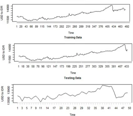
[image:6.612.310.523.515.702.2]

As explained in the previous session that the data used in the study is the USD daily middle exchange rate data against IDR period January 2, 2014 - December 31, 2015. The data plot is presented in Figure 2.

(7)

4459 Based on Figure 2, it is known that the exchange rate of USD to IDR tends to increase, which means that Rupiah (IDR) tends to depreciate by US Dollar (USD). The lowest exchange rate occurred on April 1, 2014, with a value of Rp11,271.00. The rupiah fell on September 29, 2015, with a value of Rp14,728.00. According to Rachbini (in Suryowati, 2015), the sinking of rupiah value is caused by economic factors and non-economic factors. Some non-economic factors that make up the value of rupiah are political factors and social factors. Inadequate internal relations among officials indicate that the leadership factor in Indonesia is still weak. Another non-economic factor is the lack of public confidence in the rupiah. On the other hand, some economic factors affecting rupiah are export developments that have not shown any signs of recovery, lack of monetary authority initiatives, and late-issued policy packages. Rupiah strengthened again in the range of Rp13,000.00 on October 8, 2015, then exchange rate fluctuated until the end of 2015.

The number of observation in the period January 2, 2014 - December 31, 2015, with the provisions of the observation of the effective day of work is 489 points. There is no definite provision regarding the distribution of training and testing data. In this research, the data of training and testing is determined by considering the data pattern. There is an extreme pattern change in the period September - October 2015, so the proportion is set at 90%: 10%. Modeling is done on the first 440 observations (January 2, 2014 - October 20, 2015) and the remaining 10% (October 21, 2015 - December 31, 2015) is used s data testing. The training and testing data sharing plot is shown in Figure 1.

Data testing is used to check the sustainability of time series patterns. Models formed from the exchange rate of USD to IDR on training data are used to predict the exchange rate of USD to IDR on training and testing data. If the model is able to predict the exchange rate in training and testing data accurately then the model can be said to be good. Thus the best model criterion is a model that is able to predict the exchange rate on the training data and mainly on the testing data accurately.

4.1.Identify FIS inputs and arrange tentative models

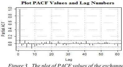
In the research identification of input-model is done by using partial autocorrelation

[image:7.612.317.515.202.311.2]

coefficient plot (PACF). PACF is used as an input identification tool for the reason that PACF describes the autoregression process. The confidence level used to test the PACF is 95%, so the test confidence limits are ± 2 / √440 = ± 0.0953. The PACF plot of the exchange rate of USD to IDR on training data and the PACF value of the first 15 lags is presented in Figure 3.

Figure 3. The plot of PACF values of the exchange rate of USD to IDR on training data

Based on the plot of PACF in Figure 3 it is known that the PACF values are significant in lag 1, lag 5, lag 8, and lag 10. It can be seen that PACF value lag 1 is close to 1, it shows that there is a very strong dependence between and (linear trend). In this study, denotes the exchange rate of USD to IDR on day t. The identification results indicate that the maximum significant lag is lag 10, so the maximum lag considered is 10 , the observation index for output starts from the

11-th period .

The tentative models are determined based on a combination of 2 inputs, 3 inputs and 4 inputs of significant lag and the number of clusters or fuzzy sets as 3, 5 and 7. Although the identification results show that lag 1, 5, 8, and 10 are significant, defined as a tentative model is a combination that includes lag 1. Considering that there is a strong dependence between and . Table 1 shows the tentative models specified.

Table 1. The Tentative Models of the Combination between Inputs of 2, 3, 4 and Linguistic Values of 3, 5, 7

Model Inputs Number

Input Variables Name

Clusters Number 1

Two input variables

(3,3)

2 (5,5)

3 (7,7)

4 (3,3)

5 (5,5)

6 (7,7)

7 (3,3)

(8)

4460

9 (7,7)

10

Three input variables

(3,3,3)

11 (5,5,5)

12 (7,7,7)

13 (3,3,3)

14 (5,5,5)

15 (7,7,7)

16 (3,3,3)

17 (5,5,5)

18 (7,7,7)

19

Four input variables

(3,3,3,3)

20 (5,5,5,5)

21 (7,7,7,7)

Based on Table 1, the number of tentative models is 21 models. The tentative models are classified into 3 groups, ie models with 2 input variables, 3 input variables, and 4 input variables. The selection of the best model will be done in each group and will be selected one best model from the best. The precision of the model is assessed using MAPE and R2_{. To provide an overview and understanding of} the formation of Fuzzy Takagi-Sugeno system based on FCM-PSO, then in the following session given detailed exposure of the system with 2 input variables and 3 fuzzy sets.

4.2.Implementation FIS of Takagi-Sugeno with Optimal Rule Bases

As an illustration, we will take one of the tentative models with the input variables and the number of clusters of (3.3). Modeling will be done gradually, starting from clustering with FCM, estimating the spread parameter with PSO and consequent parameter estimation.

[image:8.612.84.306.82.247.2]

The clustering input-output aims to group output pairs into multiple clusters. The input-output pairs will be grouped into (3.3) clusters. The main purpose of applying clustering with FCM is to obtain center of clusters and partition matrices. The cluster center is used as the center parameter of gaussmf, the partition matrix is used to estimate the spread parameter of gaussmf. In accordance with the predefined input argument parameter setting of the FCM, the iteration required until it reaches the convergent is 53 iterations with the objective function of c-Means of 98981225. The cluster centers generated by FCM are presented in Table 2.

Table 2. Three Cluster Centers of Two Input Variables

Cluster

label Variable name

1 11810.27 11808.32 11811.47

2 13023.32 12996.36 13030.67

3 14185.03 14151.11 14183.8

The center (middle value) variables and in each cluster are used as the center parameters of gaussmf for input variables. The middle value of the variable is not used, because the consequent part of the fuzzy rule base of the Fuzzy Takagi-Sugeno inference model is not a fuzzy set, but a linear equation. The partition matrix is a matrix whose elements are the degree of input-output pair membership in each cluster. The degree of input-output pair membership in each cluster is presented in Table 3.

Table 3. The Degree of Membership of Each Input-Output Pairs

Cluster

Label 1 2 Time period (t) 3 4 ... 440

1 0.82 0.85 0.90 0.88 ... 0.05

2 0.15 0.13 0.09 0.10 ... 0.54

3 0.03 0.02 0.02 0.02 ... 0.41

The memberships of the input-output pair in each Cluster are indicated by the highest degree of membership. As an example for t = 11, the highest degree of membership lies in cluster 1, so the input-output pairs for t = 11 become the member of cluster 1.

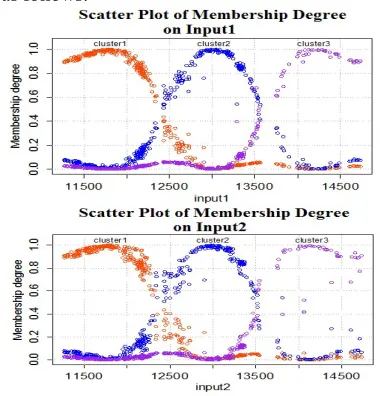
[image:8.612.309.528.264.326.2]

The fuzzy set (gaussmf) is formed through fitting which is done between the input variables and the degree of input-output membership in each cluster. The scatter plots between and each degree of membership in each cluster are shown in the Figure 4 as follows:

Figure 4. The Scatter plots of the degree of membership of the input variables on each cluster

[image:8.612.320.510.487.685.2]

(9)

4461 squares of error. The scatter plot in Figure 4 forms a bell-like pattern so that the relevant gaussmf is used to approach the degree of input-output membership. The objective function for the estimated spread parameters is listed in Table 3. In each with (h = 1,2,3; k = 1,2), we will find which minimizes . The value of is searched by performing objective

[image:9.612.90.526.219.505.2]

function optimization . The specified search interval is [0, 1187.3810] for input 1 and [0, 1171.3960] for input 2. The upper limit of the search interval on each input variable is obtained from differences between the highest center cluster and lowest cluster center that divided by the number of clusters minus 1.

Table 4. The Objective Function of SSE Optimized by Using PSO

Cl.

Lab. _{Objective functon (SSE)}Input1 _{Objective functon (SSE)}Input2

1

2

3

As an example for input1, the upper limit of the interval is calculated from (14185.0300-11810.2700) / (3-1) = 1187.3810. The plot of the objective function based on the search interval is presented in Figure 5.

Figure 5. Plot of the optimal SSE objective function on three clusters and two input variables

Based on the plot of the objective function in Figure 5, the which minimizes

[image:9.612.81.521.593.689.2]

lies between 400 and 600. The optimization results of each objective function are presented in Table 5 as follows:.

Table 5. The Results of PSO Optimization on SSE Objective Function

Cluster

Label

Input1

Input2

Objective function

Iterat.nu mbers

Object. value

Stoping Condit.

Objective function

Iterat. Nnumb.

Object. value

Stoping Condit.

1 525.0

4 98 2.8852 0.0003

512.2

7 68 3.9744 0.0005

2 463.3

4 98 1.4471 <0.0001 460.74 98 2.7242 0.0005

3 463.1

7 98 1.8384 0.0002

463.2

3 98 2.417 <0.0001

Table 5 shows that the optimization of each objective function has a different convergence. The convergence difference is indicated by the number

(10)

[image:10.612.94.292.82.331.2]

4462

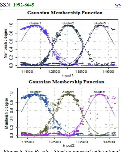
Figure 6. The Results fitted on gaussmf with optimal spread parameters

[image:10.612.86.497.400.637.2]

The Gaussmf parameters that are the antecedent parts of the rule bases are presented in Table 6

Table 6. The Estimation Values of Spread Parameters of Gaussmf

Rule Label

Input1 Input2

1 11810 525 11808 512

2 13023 463 12996 460

3 14185 463 141511 463

The antecedent part of the rule will be used to input fuzzification process. The fuzzification stage will be continued by calculating the normalized fire strength. For each input-output pair, the input part will be used to form the input matrix, while the output part will be organized into an output vector. The input matrix is seen as the observed value of a predictor, while the output vector is seen as the observed value of the response variable. Therefore a combination of input matrix and output vector can be viewed as a linear system. The coefficients of each predictor variable can be obtained by applying OLS optimization so that the result of the consequence parameter estimation as shown in Table 7.

Table 7. The Estimation of The Consequent Coeficiences

Rule Conseq.

1 101.52 0.99 -0.0042

2 221.19 0.85 0.1349

3 1702.04 1.10 -0.2241

In accordance with the result of the coefficient estimation of the linear equation which is the consequent part of the fuzzy rule bases, the Fuzzy Takagi-Sugeno model with the input and the number of clusters of the input variables (3.3) are as follows:

Where,

, , ,

The model formed from training data in the period t = 11.12, ..., 440 is a model of the FIS with 2 input variables and each input is divided into 3 fuzzy sets. Next, the Input variable pair is used to calculate the exchange rate of USD to IDR of the t period for t = 11.12, ..., 440 and for t = 441.442, ..., 489 ie periods in both

(11)

4463

4.3. The Best Model of the Takagi-Sugeno FIS with FCM and PSO optimization

The best model selection is done in 2 stages. The selection in the first stage is done in each group (based on the number of input

[image:11.612.140.472.192.474.2]

variables), so that in the first phase it is resulted 3 models selected, then it will be continued to select the best model. A measure of the accuracy of a tentative model in both training and testing data is presented in Table 8 as follows:

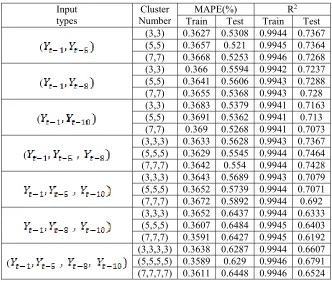
Table 8. Both MAPE and R2_{indicators of 21 FISs in both training and testing data}

Input types

Cluster Number

MAPE(%) R2

Train Test Train Test

(

(3,3) 0.3627 0.5308 0.9944 0.7367 (5,5) 0.3657 0.521 0.9945 0.7364 (7,7) 0.3668 0.5253 0.9946 0.7268

(

(3,3) 0.366 0.5594 0.9942 0.7237 (5,5) 0.3641 0.5606 0.9943 0.7288 (7,7) 0.3655 0.5368 0.9943 0.728

(

(3,3) 0.3683 0.5379 0.9941 0.7163 (5,5) 0.3691 0.5362 0.9941 0.713 (7,7) 0.369 0.5268 0.9941 0.7073

(

(3,3,3) 0.3633 0.5628 0.9943 0.7367 (5,5,5) 0.3629 0.5545 0.9944 0.7464 (7,7,7) 0.3642 0.554 0.9944 0.7428

(3,3,3) 0.3643 0.5689 0.9943 0.7079 (5,5,5) 0.3652 0.5739 0.9944 0.7071 (7,7,7) 0.3672 0.5892 0.9944 0.692

(3,3,3) 0.3652 0.6437 0.9944 0.6333 (5,5,5) 0.3607 0.6484 0.9945 0.6403 (7,7,7) 0.3591 0.6427 0.9945 0.6192

(

(3,3,3,3) 0.3638 0.6287 0.9944 0.6607 (5,5,5,5) 0.3589 0.629 0.9946 0.6791 (7,7,7,7) 0.3611 0.6448 0.9946 0.6524 The model is said to be good if both

MAPE and R2_{values are optimum that means the} small MAPE value (toward 0) and the high R2 value ( close to 1) both in the training data, and in the testing data. In the study, both of the indicators of model goodness are considered in both training and testing data in order to see the consistency of model capability in predicting USD to IDR exchange rate, as shown in Table 8, although not significant, the additional number of clusters tends to increase R ^ 2 training period. However, an increase in R ^ 2 does not always apply to testing data. So that with many clusters does not guarantee that the model is able to predict the exchange rate of USD to IDR accurately. Based on both the MAPE and R ^ 2 indicators presented in Table 7, the following information can be obtained:

a. The best model of FIS FCM-PSO with 2 input variables.

MAPE and R2_{are optimally respectively for} the model with 2 input variables is 0.3657%, and 0.9945 in the training data, whereas in the

data testing the value of MAPE and R2_are 0.5210% and 0.7364 respectively. This value represents the MAPE and R2_{values of the} model with the inputs and the cluster as much as (5,5) respectively.

b. The best model of FIS FCM-PSO with 3 input variables.

MAPE and R2_{are optimally respectively for} models with 3 input variables is 0.3629%, and 0.9944 in training data, whereas in data testing the value of MAPE and R2 are 0.5545%, and 0.7464 respectively. The value is MAPE and R2 _of _the _model _with _input

and cluster as much as (5,5,5) respectively.

c. The best model of FIS FCM-PSO with 4 input variables.

In this study, the model with 4 input variables is a model that includes all significant PACF lags as

inputs, ie . The

(12)

4464 0.3589%, and 0.9946, respectively. While in the data testing the value of MAPE and R2_{are 0.6290%} and 0.6791 respectively. This value represents the MAPE and R2_{values of the model with the cluster} as much as (5,5,5,5) respectively.

The values of the optimal MAPE and R2 indicators of the three consecutive model groups were 0.3657%, and 0.9945 for training data, while in the testing data were 0.5210% and 0.7364. This value represents the MAPE and R2_{values of the} model with the inputs and the cluster as much as (5,5). So the best FCM-PSO Fuzzy Takagi

Sugeno model to predict the exchange rate of USD to IDR is the model with input and cluster as much as (5,5) respectively.

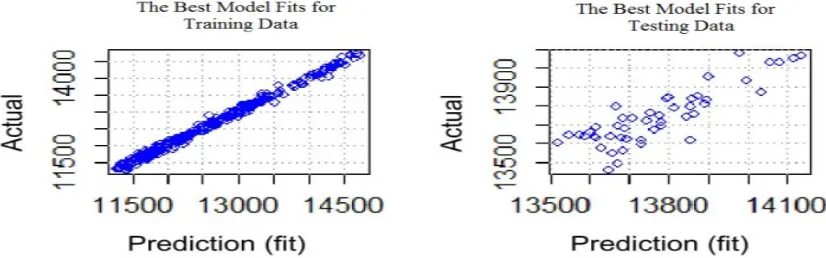
[image:12.612.101.514.241.370.2]

Both the actual and predictive values comparison plots are used to visually view the model's accuracy. A good model is a model that can approach the actual value accurately. Visually demonstrated by predictive plot values close to the actual values. Plots used to describe model accuracy are scatter plots and time series plots, each of which is presented in Figure 6 and Figure 7.

Figure 7. The Scatter plot of both actual and predictiive values of the best model in both training and testing data

The left side of Figure 7 states the scatter plots of training data where it is apparent that the predicted values and actual values form a straight line pattern. This confirmed the value of R2_{from the best model} in the training data of 99.45%. While on the right

[image:12.612.92.515.462.633.2]

side of Figure 6 states plots in the data testing in which the linear pattern is formed also seems quite clear, but there is still a rather wide gap. Thus very reasonable if the value of R2_{of this best model in} the testing data of 73.64%.

Figure 8. Time series plots of actual versus prediction values of the best model in both training and testing data

The plot located to the left of the vertical line in Figure 8 states the plot of the actual value versus the predicted value of the training data. In this case the best model is able to capture all the patterns in the training data with almost perfect so that the R2 value of 99.45% and MAPE value of 0.3657%. while the plot of data testing shown by the right of

(13)

4465

5. CONCLUSION

The selection of input variables with identification through PACF resulted in FIS Takagi Sugeno based on FCM and PSO that performed almost perfectly on training data where the R2_was between 98.89% and 99.45%, and the MAPE was all of close to 0.36%.The FIS performances in the testing data were varied with a considerable range. The selection of number of clusters and number of inputs has a positive trend towards system performance. The greater number of clusters and the more number of input variables will be followed by the increasing of R2_{values and the decreasing of} MAPE values in the training data. The very different results are seen in the testing data where there is a negative trend. The performance of the system decreases if both number of clusters and number of input variables increase. The best performance of FCM-PSO of Takagi-Sugeno FIS model for forecasting the USD to IDR exchange rate data is a model which has the inputs of (Yt-1, Yt-5) and the number of clusters of (5.5). The best model has both MAPE and R2_{in the training data are 0.36% and} 99.45% respectively, and both MAPE and R2_{in the} testing data are 0.52% and 73.64% respectively.

REFRENCES:

[1] A. Widodo and S. Handoyo, “The

Classification Performance Using Logistic Regression And Support Vector Machine (Svm)”, Journal Of Theoretical & Applied

Information Technology, 95(19), 2017, pp:

5184-5193.

[2] WH. Nugroho, S. Handoyo, and YJ. Akri, “An

Influence of Measurement Scale of Predictor Variable on Logistic Regression Modeling and Learning Vector Quntization Modeling for Object Classification”, International Journal of

Electrical and Computer Engineering (IJECE),

8(1), 2018, pp: 333-343.

[3] Babu CN, Reddy BE, “A moving-average filter

based hybrid ARIMA–ANN model for forecasting time series data”, Applied Soft

Computing, 2014, pp. 23: 27-38.

[4] H. Kusdarwati, and S. Handoyo, “System for Prediction of Non Stationary Time Series Based on the Wavelet Radial Bases Function Neural Network Model”, International Journal of Electrical and Computer Engineering

(IJECE), 8(4), 2018, pp: 2327-2337.

[5] Nayak PC, Sudheer KP, Rangan DM,

Ramasastri KS, “A neuro-fuzzy computing technique for modeling hydrological time

series”, Journal of Hydrology, 29(1-2), 2004, pp: 52-66.

[6] Vairappan C, Tamura H, Gao S, Tang Z,

“Batch type local search-based adaptive neuro-fuzzy inference system (ANFIS) with self-feedbacks for time-series prediction”,

Neurocomputing, 72(7-9), 2009, pp:

1870-1877.

[7] Esfahanipour A, Aghamiri W, “Adapted

neuro-fuzzy inference system on indirect approach TSK fuzzy rule base for stock market analysis”, Expert Systems with Applications, 37(7), 2010, pp: 4742-4748.

[8] F Arci, J. Reilly, P. Li, K. Curran, and A. Belatreche, “Forecasting Short-term Wholesale Prices on the Irish Single Electricity Market”, .

International Journal of Electrical and

Computer Engineering (IJECE), 8(6), 2018,

pp. 4060-4078.

[9] HM. Rahman, N. Arbaiy, R. Efendi, and CC. Wen, “Forecasting ASEAN countries exchange rates using auto regression model based on triangular fuzzy number”, Indonesian Journal of Electrical Engineering and Computer

Science (IJEECS), 14(3), 2019, pp: 1525-1532.

[10] Cryer JD, Chan KS, Time series regression models. Time series analysis: with applications in R, New York: Springer. 2008: 249-776.

[11] Montgomery DC, Jennings CL, Kulahci M.

Introduction to time series analysis and

forecasting. New York: John Wiley & Sons.

2015.

[12] Wang LX, Mendel JM. “Generating fuzzy

rules by learning from examples”. IEEE Transactions on systems, man, and cybernetics,

22(6), 1992, pp: 1414-1427.

[13] Nozaki K, Ishibuchi H, Tanaka H. “A simple but powerful heuristic method for generating fuzzy rules from numerical data”. Fuzzy sets

and systems, 86(3), 1997, pp: 251-270.

[14] MF. Arif, B. Anoraga, S. Handoyo, and H. Nasir. “Algorithm Apriori Association Rule in Determination of Fuzzy Rule Based on Comparison of Fuzzy Inference System (FIS) Mamdani Method and Sugeno Method”.

Business Management and Strategy, 7(1),

2016, pp: 103-124.

[15] A. Priyono, M. Ridwan, A.J. Alias, R.A. Rahmat, A.Hassan, M.A. Ali. “Generation of fuzzy rules with subtractive clustering”. Jurnal

Teknologi, 43(1), 2012, pp: 143-153.

(14)

4466 segmentation”. Pattern recognition, 40(3), 2007, pp: 825-838.

[17] S. Handoyo, Marji, IN. Purwanto, and F. Jie. “The Fuzzy Inference System with Rule Bases Generated by using the Fuzzy C-Means to Predict Regional Minimum Wage in Indonesia”. International J. of Opers. and

Quant. Management (IJOQM), 24(4), 2018,

pp: 277-292.

[18] S. Handoyo, and Marji. “The Fuzzy Inference System with Least Square Optimization for Time Series Forecasting”. Indonesian Journal of Electrical Engineering and Computer

Science (IJEECS), 7(3), 2018, pp: 1015-1026.

[19] Del Valle Y, Venayagamoorthy GK,

Mohagheghi S, Harley RG, Hernandez JC. “Particle swarm optimization: basic concepts, variants and applications in power systems”.

IEEE Transactions on evolutionary

computation, 12(2), 2008, pp: 171-195.

[20] Kennedy J. Particle swarm optimization. In

Encyclopedia of machine learning. New York:

Springer. 2011, pp: 760-766.

[21] S. Handoyo, A. Efendi, F. Jie, and A. Widodo. “Implementation of particle swarm optimization (PSO) algorithm for estimating parameter of arma model via maximum likelihood method”. The Far East Journal of

Mathematical Sciences(FJMS), 102(7), 2017,

pp: 1337-1363.

[22] Chen G, Pham TT. Introduction to fuzzy sets,

fuzzy logic, and fuzzy control systems. New

York: CRC Press. 2000.

[23] S. Handoyo, and A.P.S. Prasojo. Applied Fuzzy System with R Software (Sistem Fuzzy terapan

dengan Software R). Malang: UB Press. 2017.

[24] Palit AK, Popovic D. Computational

intelligence in time series forecasting: theory

and engineering applications. London: Science

& Business Media. Springer. 2006.

[25] Wang LX. A Course Fuzzy Systems and