A HYBRID METHOD OF LINGUISTIC APPROACH AND STATISTICAL METHOD FOR NESTED NOUN COMPOUND EXTRACTION

(1)

EMPIRICAL FACTORS FOR ROBUSTNESS OF SENSOR

NODES ON ENERGY EFFICIENCY

1_{Prof. T.P. JAYAKUMAR ,} 2_{Dr. N. GUNASEKARAN}

1

Associate Professor /CSE, Maharaja Engineering College for Women, Perundurai, Tamilnadu, India.

2

Principal, SNS College of Engineering, Coimbatore, Tamilnadu, India. E-mail: 1 [email protected], 2 [email protected]

ABSTRACT

Sensors are the devices which are used to measure the temperature of their surroundings and inform it to the base station through central heads which forms large scale networks, have become more in number. These sensors can act individually by using small hardware devices and it can be embedded into the devices like mobile phones, laptops, iPods, or in combination of these in Mobile Ad-hoc Networks (MANETs) more battery power is needed for the measurement of temperature. Depending on the rate of battery power consumption, more research works are being focused on the influence of data processing and communication network as these sensors are tiny and they cannot withhold larger batteries. The problem arises when the sensors are treated as either tiny stand alone devices or particularly used when it is embedded with robust devices. It is necessary to make research work on embedded devices. Even though the literature shows the effectiveness of energy consumption by sensors, studies on the embedded devices robustness are seen rarely. It is being pointed out by architectural design of sensor networks which is different according to their applications and constraints. In order to address these issues, this paper try to arrive at certain coefficients called as factors that are empirically determined by involving series of experiments in the NS 2.0 environment. High, Medium, Low are the three scales of robustness which are suggested for the factor and also the three scales are immense to be used in the deployment of sensors in manets. Robustness on the consumption of energy of the sensor embedded devices in networks is indicated by the factors considered. The experimental work is delimited in its scope with energy consumption due to the computing process. The work is delimited to comparative studies on hierarchal and flat algorithms. Concluding remarks have been drawn out of these experimental studies.

Keywords: Manets, Central Head, Wireless Sensors, Robustness, Routing

1. INTRODUCTION AND BACKGROUND

Small-sized battery-operated sensors are capable of detecting energy sources such as temperature, sound etc. These sensors are generally embedded with communicating and computing devices. They are capable of sensing and measuring energy sources from their surrounding environment and transforming them into electric signals. Consequently they help in detecting some properties about objects located and/or events happening in the vicinity of the sensor. Therefore aggregating these capabilities of individual sensors in a large scale network can be operated unattended [1]. They can be deployed randomly in the area of interest by a relatively uncontrolled means, thereby to collectively form a network in an ad-hoc manner [2]. However, the short lifespan of the battery-operated sensors and the possibility of having

(2)

braided sensor nodes are considered for the experiments of this paper. This paper forms a part of a whole larger research. The need for the research, through the experimental studies, is to propose efficient schema of the braided sensor nodes and appropriate routing algorithmic procedures that consider three categories of varying transmitting powered sensor nodes. The varying transmitting power of the sensors would be grouped into the three categories (ranges) of robust (gradation of resilient) sensors.

Architectural designs of wireless sensor networks would be different according their constraints and applications. Such networks basically consist of sensor nodes, base-station and a monitor system [4]. Most of architecture of sensor networks assumes their nodes are stationary. In some architecture, the aggregated data are assigned to a Central Head that could as well be a powerful node. However in such cases these Central Heads are not over burdened, so as to facilitate them to provide accurate data efficiently [5]. An indication for parametric studies in such situations as it may be necessary to assign backup Central Heads for a cluster or it may be needed to rotate some nodes to act as the Central Head [6]. Sensor networks require low reporting rate in order to save energy [7]. Sensor nodes and their link qualities, and their capabilities around the nodes are important decisive parameters that would contribute to weights for data transmission and hence must be considered for study [9]. In the case of sensor networks having homogeneous nodes, all having equal capacity in terms of power and other attributes, then Central Head may be picked from the nodes [6] which have significantly more resources. In such case the selection is carefully tasked. Three important criteria that would drive the design of large-scale sensor networks are scalability, energy-efficiency and Robustness [11]. These networks require novel routing techniques for scalability and robust data dissemination. The paper accordingly attempts to demonstrate two selective algorithmic approaches for two situations. Literature on homogenous sensors in terms of resilience has been reported. But the present paper brings out research findings from heterogeneous nodes with the chosen three categories of resilient sensors (robustness). The ultimate objective of the paper is to bring out empirical factors that would help in identifying the optimum ratios of the chosen three categories of the robust sensors. The

analyses in the overall larger research will be carried out in three different layers and correlated with combined three categories of resilient sensor layers. However this study is beyond the scope of this paper. The paper attempts to bring out only the empirical factor for the categories for efficient combinations.

2. EXPERIMENTAL STUDIES

The aim of the proposed experiments is to determine the influencing factors of robustness of sensor nodes in Networks for computing the energy consumed by the nodes in transmitting the data to a Central Head (CH). The contribution of CH in facilitating the transmission of data for receipt to it, from the sensor nodes is considered for the experiments. This class of experiment has not to be found in literature and thus justifies the novelty of our work.

2.1 Conditional Parameters for the

Experiments

Residual energy of each hardware item of the sensor embedded node would be the primary parameter that should be considered for election of CH [4]. We have thus attempted to correlate the node’s robustness with residual energy. In view of this, three categories in the form of types of nodes grouped in lots are considered for the proposed study. These three types of nodes mentioned below are subjected to the proposed parametric study to determine the behavior of the nodes under two different kinds of algorithm for receiving and transmitting the sensor data sent by the nodes to the CH. This CH is a special node acting as the recipient of data sent by the nodes in the experimental setup. The algorithm is deployed in this CH. The three categories or types of nodes considered are:

1. High Robust system: Tightly coupled; Single functioned and Rigid systems. (Ex. Mobile phones, I_pads)

2. Low Robust system: Loosely constrained; Multi functioned and Flexible systems. (Ex. Assembled clone systems)

3. Medium Robust system: Properties and components in-between the above two. (Ex. Branded LAP TOP systems).

(3)

experiments. The number of nodes considered in lots is increased from 100 to 1000 in increment of 100, thus amounting to 10 lots for 10 experiments, as generally, the network has a large number of sensor nodes [1]. The experiments are done for two categories of routing algorithm, as per the objective of the paper, as more resilient typically consume more energy [11]. They are: i. Hierarchical routing algorithm and ii. Flat routing technique. Literature points out to the fact in determining parameters that are to be infused in the algorithm for determining energy consumptions [10]. These parameters, such as power and hops, need to be used in mathematical forms for ultimately achieving minimal energy consumption [1]. Simulated experimental results show reduction of energy levels that used such parameters [10]. This will lead to a total of 20 cases for 20 experiments. NS 2.0 package has been adapted for the experiments.

2.2 Delimitations for the Experiments

For the purpose of the proposed experiments the following delimited principles and definitions have been assumed.

1. Preference for selection of node, when multiple nodes are received by the CH, depends on the robust parameter of the particular node.

2. Euler’s geometry is not considered for exactly computing network characters and the CH is located at the central of the nodes. 3. As the experiments are meant for the study

of behavior of nodes of three categories only, dynamic behavior of nodes of Networks is not considered for the experimental studies.

4. The data transmitted time on receiving from nodes by the CH is only the processing time by the CH and the network travel time and retention time in nodes are not considered. Because, no routing protocol could have the prior knowledge of the actual path of data traffic and how the pattern would be [8]. 5. The battery power consumed by a node is

proportional to the data transmission time consumed by the node. Other criteria like mobility of nodes are not considered by the study.

6. Fixed uniform packet sizes have been considered for transmitting from all the nodes at a time for the experiments.

7. Hierarchical routing philosophy refers to grouping of routers together by function into a hierarchical table. Flat routing technique refers to the fact that no efforts are made to organize the traffic or network routing preference; instead data transmitted first cum first basis.

3.RESULTS AND DISCUSSIONS

For the purpose of determining the contribution of hierarchical routing algorithm, which is based on grouping different types of nodes under the selected three robust types, the energy consumption of individual node is computed as under.

The battery power consumed after a time interval of ‘t’ Secs. by a node: BP (t) ---(1) It is delimited that the power consumption by battery is directly proportional to the data transmitting time taken by the node.

Rc = Category number of the node (1 to 3) ----(2)

Tj = Total number of nodes in corresponding

category (j) --- (3)

Data transmitted time by each node = Tt (i, j)

---(4)

Where i = 1 to Rc (Equ. (2)) of corresponding

node category and j = 1 to Tj of equ. (3).

Virtual Time consumed by a node for battery power Vt (i,j)= α (i) * Tt (i,j) --- (5)

Where α (i) is an empirical factor determined by parametric study for each category and Tt (i,j) of

equ. (4) for the ‘t’ of equ. (1).

(4)

[image:4.595.84.525.96.774.2]

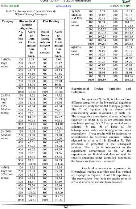
Table 1.0: Average Data Transmitted Time By Different Routing Techniques

Category Hierarchical

Routing Algorithm Flat Routing No. of Nod es Avera ge Data Trans mitted time in Secs. No. of Nodes having only one category of sensors Avera ge Data Trans mitted time in Secs. 1)100% High robust

100 9.58 100 9.01 200 21.02 200 20.12 300 31.56 300 29.66 400 43.33 400 41.13 500 54.10 500 50.16 600 65.00 600 63.23 700 76.78 700 75.08 800 88.06 800 86.86. 900 97.98 900 96.68 1000 105.45 1000 101.15 2) 50% High and 50% Medium robust

100 11.02 100 17.92 200 24.04 200 20.09 300 36.46 300 56.36 400 47.34 400 49.54 500 59.91 500 97.91 600 72.71 600 76.71 700 84.02 700 89.72 800 97.98 800 97.18 900 104.43 900 114.48 1000 123.23 1000 129.43 3) 100%

Medium robust

100 10.04 100 10.01 200 21.00 200 21.00 300 30.09 300 30.09 400 42.21 400 41.27 500 53.23 500 51.28 600 64.02 600 63.09 700 75.51 700 74.56 800 85.98 800 85.98 900 97.21 900 98.29 1000 108.88 1000 104.08 4)50%

High and 50% Low robust

100 11.32 100 14.34 200 25.08 200 29.28 300 38.64 300 44.44 400 49.84 400 38.14 500 61.61 500 66.69 600 75.76 600 85.16 700 88.92 700 88.12 800 105.98 800 115.00 900 110.63 900 115.63 1000 128.43 1000 141.43

5) 50% Medium and 50% Low robust

100 17.23 100 12.13 200 38.05 200 22.13 300 52.46 300 42.46 400 91.31 400 101.31 500 111.17 500 117.12 600 132.22 600 130.22 700 156.72 700 158.12 800 169.23 800 169.13 900 185.34 900 189.33 1000 199.63 1000 209.63 6)100%

Low robust

100 10.24 100 13.24 200 21.07 200 23.17 300 31.29 300 32.29 400 41.21 400 41.91 500 53.23 500 55.27 600 65.92 600 67.92 700 75.54 700 79.04 800 88.08 800 88.98 900 98.21 900 101.26 1000 108.89 1000 108.32

Experimental Design Variables and

Definitions

In Equation (2), the Rc is taken as three

different categories by the hierarchical algorithm where as it is unity for the flat routing algorithm. The Tj of Equation (3) is shown with

corresponding values in column 1 of Table 1.0. The average data transmission time as defined in Equation (3) under Tt (i, j), are obtained from

simulation package NS 2.0 are presented under columns (3) and (5) of Table 1.0 for heterogeneous nodes and homogeneous nodes respectively. These results will be subjected to normalization to determine empirical factors (denoted as so as α (i) in Equation 5). This procedure is presented in the subsequent sections. This α (i) is independent in the experiments demonstrated so far. As the experiments are limited and demonstrated for specific situations under controlled conditions, the factors are termed as ‘Empirical’.

(5)

Figure 1.0 Distribution Of Data Transmission Time By Systems Of Different Nodes Under

Hierarchical Routing Algorithm

Observation:

[image:5.595.88.294.130.267.2]

But for the 50% Medium and 50% Low robust systems, the rest are almost linearly distributed in consuming energy (Figure 1.0). As low and medium robust combined systems are highly un-defined in their behavior, the distribution shown is perhaps highly deviating from the rest. It is therefore inferred that the cluster is recommended to be mostly representative of uniform configuration.

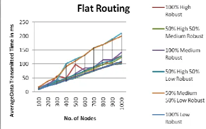
Figure 2.0 Distribution Of Data Transmission Time By Systems Of Different Nodes Under Flat

Routing.

Observation:

For the purpose of comparison, the parameters are replicated with hierarchical (heterogeneous) situation, as 50%High 50% Medium etc. But in all the situations, corresponding sensors such as ‘High’/’Medium’/’Low’ robust sensors are

considered as homogeneous for ‘Flat’ routing algorithm.

Compared with hierarchical routing algorithm, flat routing is erratic in the behavior, as seen from Figure 2.0. As there is no table that holds different types of systems, the routing is done first cum first basis.

3.1 Factor analysis

Table 1.0 presents average data transmitted time in Secs. by the two routing techniques for the two situations narrated in the experimental design below. The overall average transmitted time is computed as below for both the techniques.

Hierarchical Routing algorithm:

This routing algorithm is suggested for combined presence of the three categories of sensors (heterogeneous). The average transmission time in such situation is computed through the equations demonstrated below.

Complete experimental average transmission time by category (1) = (9.58 + 21.02/2 + 31.56/3 + 43.33/4 + 54.10/5 + 65.00/6 + 76.78/7 + 88.06/8 + 97.98/9 + 105.45/10) / 100 = 0.11774 Secs. = 117.74 ms.

Complete experimental average transmission time by category (3) = (10.04 + 21.00/2 + 30.09/3 + 42.21/4 + 53.23/5 + 64.02/6 + 75.51/7 + 85.98/8 + 97.21/9 + 108.88/10) / 100

= 0.121051 Secs. = 121.05 ms. Complete experimental average transmission time by category (4) = (11.32 + 25.08/2 + 38.64/3 + 49.84/4 + 61.61/5 + 75.76/6 + 88.92/7 + 105.98/8 + 110.63/9 + 128.43/10) /100 = 0.14240 Secs. = 142.40 ms.

[image:5.595.88.297.465.596.2]

(6)

Flat Routing:

This routing algorithm is suggested for the presence of any one category of the sensors (homogeneous). The average transmission time in such situation is computed through the equations demonstrated below.

Complete experimental average transmission time by category (3) = (10.01 + 21.00/2 + 30.09/3 + 41.27/4 + 51.28/5 + 63.09/6 + 74.56/7 + 85.98/8 + 98.29/9 +104.08/10) / 100 = 0.11637 Secs. = 116.37 ms. Complete experimental average transmission time by category (4) = (14.34 + 29.28/2 + 44.44/3 + 38.14/4 + 66.69/5 + 85.16/6 + 88.12/7 + 115.00/8 + 115.63/9 + 141.43/10) /100 = 0.15608 Secs. = 156.08 ms

3.2 Normalization of Factors

From normalization out of averaging with pairs of α (1) and α (2), α (1) and α (3) α (2) and α (3) using numerical methods, the empirical values for robust categories after normalization, are:

Hierarchical Routing algorithm:

α (1) = 127.74 ms; ratio with respect to α (1) = 1.00.

Flat Routing:

Empirical factors are arrived with respect to the base, which is fully robust from the average value of both the routing techniques. The final empirical values thus arrived at are:

For robust nodes α (1) = 1.0. For semi robust nodes α (2) = 1.23. For non robust nodes α (3) = 1.25. The virtual time of data transmission by nodes, is determined from Equ. 5, by applying respective α values. Equation 1 will provide the virtual energy efficiently consumed by the nodes.

4. CONCLUSION AND FUTURE SCOPE

The results will be of immense use to researchers in the field of optimizing braided resilient sensor network for energy saving. The two algorithms suggested by the research are to be applied (i) hierarchical routing algorithm for combined layer situation (heterogeneous resilient sensors) and (ii) flat routing algorithm for single layer situation (homogeneous resilient sensors). The three empirical factors indicate the optimum ratios of resilience features of the sensor categories along with suitable routing algorithms (for multi layer as well as single layer) for implanting in the braided sensor networks so as to achieve minimum energy consumptions of the overall network.

The experiments and the results show that suitable routing algorithm and robustness’s of sensor nodes or sensor embedded nodes would be sensitive with respect to transmission time leading to energy consumption by the nodes, even though an established hierarchical algorithm compared with traditional flat technique. The experiments also prove that grouping of sensor nodes according to levels of robustness would organize large number of sensors in network for better managements.

(7)

efficient algorithm specific for specific situations need to be incorporated that takes robustness into account. The overall power consumption by nodes increased from higher robustness to lower robust nodes in both the cases of ‘Hierarchical routing algorithm’ as well as ‘Flat routing’.

The future work will be extended with computation of probability values of success/failure rates of sensor nodes in different braided situations. For the two situations namely homogeneous and heterogeneous resilient sensors, conditional probability with ‘Naïve Bayes’ theorem would be applied, as each category of robustness will be conditional in playing the corresponding power transmission rates in the network.

REFERENCES

[1] Abbasi A. A, Younis, M. Fand Baroudi, U.A (2013), “Recovery from a Node Failure in Wireless Sensor-Actor Networks with Minimal Topology Changes”, IEEE Transactions on Vehicular Technology, Vol. 62, No. 1, pp. 256-271.

[2] K. Sohrabi et al., (2000), “Protocols for self-organization of a wireless sensor network”, IEEE Personal Communications, Vol. 7 No.5, pp 16–27.

[3] R. Burne, et. al., (2000), “A self-organizing, cooperative UGS network for target tracking”, Proceedings of the SPIE Conference on Unattended Ground Sensor Technologies and Applications II, Orlando Florida.

[4] Younis O, Fahmy S. (2004), “HEED: a Hybrid, Energy-Efficient, Distributed Clustering approach for Ad Hoc sensor networks”, IEEE Transactions on Mobile Computing, Vol 3, No. 4, pp 366-379. [5] Gupta G, Younis M, (2003), “Load

Balanced Clustering in Wireless Sensor Networks”, Proceedings of the International Conference on Communication (ICC 2003), Anchorage, Alaska,

May 2003.

[6] Heinzeman, W.B, Chandrakasan, A.P, Balakrishnan M, (2002), “Application Specific Protocol Architecture for Wireless Micro-sensor Networks”, IEEE Transactions on Wireless Network Vol.:1 Issue: 4.

[7] Tang, L, Wang, K.C and Huang, Y (2013), “Study of Speed-dependent Packet error rate for Wireless Sensor on Routing

Mechanical Structures”, IEEE Transactions on Industrial Informatics”, Vol. 9, No. 1, pp. 72-80.

[8] Chen, Y.S and Lin Y.W, (2013), “Mobicast Routing Protocol for Underwater Sensor Networks”, IEEE Sensor Journal, Vol. 13, No. 2, pp. 737-749.

[9] Pan, Z, Yang, Y and Gong, D, (2010), “Distributed Clustering Algorithms for Lossy Wireless Sensor Networks”, Network Computing and Applications, NCA, pp. 36-43.

[10]Banerjee, S and Khuller, S, (2001), “A Clustering Scheme for hierarchical Control in Multi-hop Wireless Networks”, Proceedings of 20th Joint Conference of the IEEE Computer and Communications Societies. INFO – COM’01. Anchorage, A.K.