AN ENHANCED RULE APPROACH FOR NETWORK INTRUSION DETECTION USING EFFICIENT DATA ADAPTED DECISION TREE ALGORITHM

ISSN: 1992-8645 www.jatit.org E-ISSN: 1817-3195

SMALL SIGNAL ANALYSIS OF FLEXIBLE AC

TRANSMISSION SYSTEM USING INTERLINE

POWER FLOW CONTROLLER (IPFC)

1_{CH. VENKATA KRISHNA REDDY,} 2 _{K.KRISHNA VENI,} 3_{G.TULASIRAM DAS,} 4_SIRAJ

1_{Asst. Prof., Department of EEE, CBIT, Gandipet, Hyderabad, India} 2 _{Prof., Department of EEE, CBIT, Gandipet, Hyderabad, India}

3

Prof., Department of EEE, JNTUH, Hyderabad, India

4 _{ME, Department of EEE, CBIT, Hyderabad, India}

E-mail: [email protected]

ABSTRAC

The Interline Power Flow Controller (IPFC) is a voltage-source-converter (VSC)-based flexible ac transmission system (FACTS) controller which can inject a voltage with controllable magnitude and phase angle at the line-frequency thereby providing compensation among multiple transmission lines. In this paper, the use of the IPFC based controller in damping of low frequency oscillations is investigated. An extended Heffron-Phillips model of a single machine infinite bus (SMIB) system installed with IPFC is established and used to analyze the damping torque contribution of the IPFC damping control to the power system. The potential of various IPFC control signals upon the power system oscillation stability is investigated a using controllability index. The effect of this damping controller on the system, subjected to wide variations in loading conditions and system parameters, is investigated. Results of simulation investigations in Matlab are presented to validate the proposed approach.

Key words — FACTS, IPFC, Damping, Small Signal Stability

NOTATIONS:

A

P

: transferred power of primary line,

B

P

: transferred power of secondary line,

e

P

: Total transferred power of lines,

s

V

: Terminal voltage of generator,

id

I

: Direct axis current of line i,

C : dc link capacitance

H : inertia constant (M = 2H)

i

m

: Modulation index of series converter

i

δ

: Phase angle of series converter voltage

b

V

: Infinite bus voltage

dc

V

: Voltage at dc link

t

V

: Terminal voltage of the generator

d

X

'

: Direct axis transient synchronous

reactance of generator

A

K

: AVR Gain

A

T

: Time constant of AVR

iq

I

: Quadrature axis current of line i,

d

X

: Direct axis steady-state synchronous

reactance of generator

q

X

:

Quadrature

axis

steady-state

synchronous reactance of generator,

t

1.INTRODUCTION

Low frequency oscillations with frequency in the range of 0.2 to 2.0 Hz are one of the results of the interconnection of large power systems. Modem power systems are stable if electromechanical oscillations occurring in each area can be damped as soon as possible. To increase power system oscillations stability, Power System Stabilizer (PSS) is a simple, effective, and economical method [1].

"Flexible AC Transmission Systems (FACTS)" technology has been proposed during the last three decades and provides better utilization of existing systems. Interesting FACTS capabilities such as power flow control, damping of power system oscillations, voltage regulation, and reactive power compensation make them a good option for effective utilization of power systems. In this paper one of the FACTS capabilities is damping inter-area oscillations that will be accurately investigated for IPFC.

Interline Power Flow Controller, which is proposed by Guygyi and etal [2] in l998, is a FACTS controller for series compensation with unique capability of power flow management between multi-lines of a substation. In the IPFC structure a number of inverters are linked together at their dc terminals. Each inverter can provide series reactive compensation, as an SSSC, for its own line. However, the inverters can transfer real power between them via their common dc terminal. This capability allows the IPFC to provide both reactive and real compensation for some of the lines and thereby optimize the utilization of the overall transmission system.

Like other FACTS elements, IPFC can be used for increasing power system stability against large and small disturbances.

In this paper the voltage of coupling capacitance between two VSC-based converters is used as a state variable. Output power of the generator is used as an input of PI controller, which creates proper amplitude modulation ratio for the secondary converter.

2.DYNAMIC MODEL OF THE SYSTEM

WITH IPFC

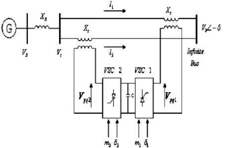
A single-machine infinite-bus (SMIB) system with IPFC, installed on two lines is considered. This configuration which consists of two parallel

[image:2.612.317.544.123.273.2]

transmission lines, connects the generator G to an infinite bus, is illustrated in figure 1.

Figure 1 Single Machine Infinite Bus System With IPFC

PSS is not taking into account in the power system. Operating conditions and parameters are represented in the appendix.

Phillips-Heffron linear model of a single-machine infinite bus system with IPFC is derived from the nonlinear differential equations. Neglecting the resistances of all the components of the system like generators, transformers, transmission lines, and series converter transformers, a nonlinear dynamic model of the system is derived as follows:

(

−

1

)

=

•

ω

ω

δ

o --- (1)

(

)

[

]

M

D

P

P

m

−

e

−

−

1

=

•

ω

ω

--- (2)

(

.

)

'

'

/

_do

fd q

q

E

E

T

E

=

−

+

•

--- (3)

(

)

[

fd A ref s

]

A

fd

E

K

V

V

T

E

=

−

+

−

/

•

--- (4)

Where,

e

P

=

P

₁+

P

₂ --- (5) e

P

=

V

_sd(

I

_1d+

V

_sq

I

_2d) + (

I

_1q+

I

_2q) --- (6)

q

E

=

E

'q+(

X

_d-

X

'd)(

I

_1d+

I

_2d) --- (7)

s

V

=

V

_sd+ j

V

_sq --- (8)

=

X

_q

I

1q+j[

E

q

'

ISSN: 1992-8645 www.jatit.org E-ISSN: 1817-3195 If the general Pulse Width Modulation (PWM) is

used for VSCs, the voltage equations of the IPFC converters in dq coordinates will be [1]:













+

























₋

=













2 2 1 1 1 1 1 1

cos

cos

2

0

0

δ

δ

m

m

V

I

I

X

X

V

V

dc q d t t q p

--- (9)













+

























−

=













2 2 1 1 2 2 2 2

sin

sin

2

0

0

δ

δ

m

m

V

I

I

X

X

V

V

dc q d t t q p --- (10) where, pqK

V

=

V

_pK + j

V

_qK=

V

_pqK

e

jδk --- (11)

[

1 1 1 1

]

1

sin

cos

4

3

_δ

_δ

q d dc

I

I

C

m

dt

dV

₌

₊

[

2 2 2 2

]

2

sin

cos

4

3

δ

δ

q d

I

I

C

m

+

+

--- (12)

From figure 1, we have:

s

V

= j

X

_s

I

_s+

V

_pq2+ j

X

_L

I

2 --- (13)

This equation in d-q coordinates is as follows:

sd

V

+ j

V

_sq= j

X

_s[(

I

_1d+

I

_2d)+j(

I

1_q+

I

2q)]+ +j

X

_L(

I

2_d+j

I

2q)+

V

p2+

V

b

sin

δ

+

jV

b

cos

δ

--- (14)

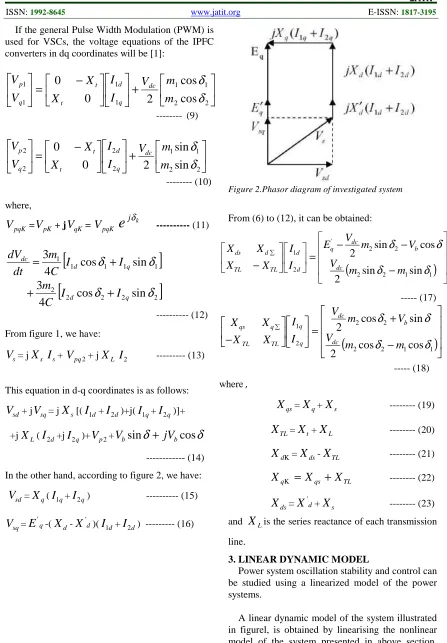
In the other hand, according to figure 2, we have:

sd

V

=

X

_q(

I

1_q+

I

2q) --- (15)

sq

[image:3.612.85.532.70.713.2]

V

=

E

'q-(

X

_d-

X

'd)(

I

_1d+

I

_2d) --- (16)

Figure 2.Phasor diagram of investigated system

From (6) to (12), it can be obtained:

(

)





















−

−

−

=

























−

∑ 1 1 2 2 2 2 ' 2 1

sin

sin

2

cos

sin

2

δ

δ

δ

δ

m

m

V

V

m

V

E

I

I

X

X

X

X

dc b dc q d d TL TL d ds

(

)





















−

+

=

























−

∑ 1 1 2 2 2 2 2 1

cos

cos

2

sin

cos

2

δ

δ

δ

δ

m

m

V

V

m

V

I

I

X

X

X

X

dc b dc q q TL TL q qs where,

X

_qs=

X

_q+

X

_s --- (19)

TL

X

=

X

_t+

X

_L --- (20)

Κ d

X

=

X

_ds-

X

_TL --- (21)

TL qs

q

X

X

X

_Κ

=

+

--- (22)

ds

X

=

X

'd+

X

_s --- (23) and

X

_Lis the series reactance of each transmission

line.

3.LINEAR DYNAMIC MODEL

Power system oscillation stability and control can be studied using a linearized model of the power systems.

A linear dynamic model of the system illustrated in figurel, is obtained by linearising the nonlinear model of the system presented in above section, --- (17)

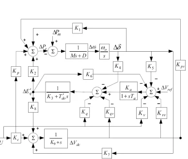
around an operating condition. The linearized model is as follows:

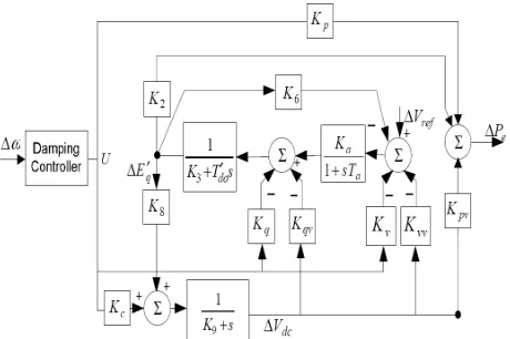
+                     ∆ ∆ ∆ ∆ ∆                       − − − − − − − − − − − =                   ∆ ∆ ∆ ∆ ∆ • • • • • dc fd q A vv A A A A A A d qv d d d pv dc fd q V E E K K K T K K T T K K T K K T K T T K T K M K M K M D M K V E E 1 9 8 7 6 5 ' ' ' 3 ' 4 2 1 1 0 0 1 0 1 0 0 0 0 0 0 ω δ ω ω δ o o o o o                 ∆ ∆ ∆ ∆                       − − − − − − − − − − − − + 2 2 1 1 2 2 1 1 2 2 1 1 ' 2 ' 2 ' 1 ' 1 2 2 1 1 0 0 0 0 δ δ δ δ δ δ δ δ δ δ m m K K K K T K K T K K T K K T K K T K T K T K T K M K M K M K M K c cm c cm A v A A vm A A v A A vm A d q d qm d q d qm p pm p pm o o o o --- (24)

In the state-space representation, the power system can be modeled as

BU

AX

X

=

+

•

Where the state vector and control vector are as follows:

T

dc fd

q

E

V

E

X

=

_



∆

δ

∆

ω

∆

'

∆

∆

_



T

m

m

U

=



_

∆

1

∆

δ

1

∆

2

∆

δ

2

_



1

m

∆

is the deviation in pulse width modulation index

m

₁ of voltage series converter-1 in line-1. By controlling

m

₁, the magnitude of series injected voltage in line-1 can be controlled.

2

m

∆

is the deviation in pulse width modulation index

m

₂ of voltage series converter-2 in line-2.By controlling

m

₂, the magnitude of series injected voltage in line-2 can be controlled.

1

δ

∆

is the deviation in phase angle of the injected voltage

V

_pq1.

2

δ

∆

is the deviation in phase angle of the injected voltage

V

_pq2.

dc

V

∆

is the deviation of coupling capacitance voltage between converters,

Using the mathematical model of the SMIB with IPFC as state space representation in (24), the

Phillips-Heffron model or linear model of the SMIB system can be obtained including IPFC [3].

Where

T

m

m

U

=

_



∆

₁

∆

δ

₁

∆

₂

∆

δ

₂

_



T

p pm p

pm

p

K

K

K

K

K

=

_



1 δ1 2 δ2

_



T q qm q qm

q

K

K

K

K

K

=

_



1 δ1 2 δ2

_



T

v vm

v vm

v

K

K

K

K

K

=

_



1 δ1 2 δ2

_



This model has 28 constants, presented below and, are functions of the system parameters and initial operating condition stated below.The system is incorporated with IPFC. Load flow analysis is performed to obtain the operating point which is given as follows:

e

P

= 0.900, Q = 0.1958

V

_s = 1.02

1

=

b

V

V

_pq1

=

0

.

3795

V

_do

=

0

.

4311

9244

.

0

=

qo

V

I

do

=

0

.

5469

I

qo

=

0

.

7185

o

6056

.

7

=

o

δ

o

o

71

.

5651

1

=

δ

o

o

7

.

725

2

=

δ

The system is linearized about this operating point. The K-constants for the system installed with IPFC, are computed as follows:

0552

.

2

1

=

K

K

₂

=

0

.

0413

7333

.

0

3

=

K

K

4

=

0

.

000001

0185

.

0

5

=

K

K

₆

=

0

.

6001

0885

.

0

7

=

−

K

K

₈

=

−

0

.

1088

4 9 7.6663 10

−

× =

K

K

pv

=

0

.

0672

0087

.

0

−

=

qv

K

K

vv

=

−

0

.

0116

0552

.

0

1

=

pm

K

K

pm2

=

0

.

2530

0376

.

0

1

=

δ p

K

K

pδ2

=

−

0

.

0045

0326

.

0

1

=

−

qm

K

K

qδ1

=

0

.

0010

0056

.

0

2

=

qm

K

K

qδ2

=

0

.

0033

0360

.

0

1

=

−

vm

K

K

vδ1

=

−

0

.

0029

0038

.

0

2

=

−

vm

ISSN: 1992-8645 www.jatit.org E-ISSN: 1817-3195

4 1

7

.

6663

10

−

×

=

cm

K

K

_cδ1

=

0

.

0672

0087

.

0

2

=

−

cm

K

K

cδ2

=

−

0

.

0116

4.DESIGN OF IPFC DAMPING

CONTROLLERS

To improve the damping of low frequency oscillations the damping controllers are provided to produce the additional damping torque. The speed

[image:5.612.97.301.273.316.2]

deviation

∆

ω

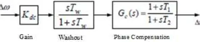
is considered as the input to the damping controllers which reflects the swings on the machines and lines of interest. As such, the output of the controller is in phase with the speed deviation.

Fig. 3 Structure of IPFC based damping controller

The structure of IPFC based damping controller is shown in Fig.3. It consists of gain, signal washout and phase compensation blocks. The optimum parameters of the damping controller are obtained using the phase compensation technique [4]. The design is presented as below. The time constants of the phase compensator are chosen such that the phase angle of the system is fully compensated. For the nominal operating condition, the magnitude and

phase angle of transfer function, ∆

P

_e/∆U, will be

computed for

s

=

j

ω

_n . The gain setting of the

damping controller is chosen to achieve the required damping ratio of 0.1. As observed from (24) there are four choices of input signals (

m

₁,

δ

₁,

m

₂and

δ

₂ ) of the IPFC to modulate. The signal which can achieve effective damping control at minimum control cost will be the most efficient. This selection is made at open loop condition before installation of damping controller. The concept of controllability index is used to select the most suitable IPFC control parameter from the damping controller for modulation [5].

(1). Compute the natural frequency of oscillation

n

ω

from the mechanical loop as

M

K

_o

n

ω

ω

=

1

(2). Let γ be the angle of the transfer function

( )

u

P

s

G

e

s

∆

∆

=

,(phase lag of between ∆u and

∆

P

_e

, where

∆

u

=

[

∆

m

₁

,

∆

δ

₁

,

∆

m

₂

and

∆

δ

₂

]

as shown in Fig.4.5, at

s

=

j

ω

_n .

(3). The controller designed is made up of washout filter and lead-lag block, with the following transfer function:

( )

2 1

1

1

1

sT

sT

sT

sT

K

s

G

w w s

+

+

⋅

+

=

w

T

is the washout filter time constant and its value

can be taken as a number between 1 and 20 sec. Assume for the lead-lag network,

T

₁

=

aT

₂ , where a = (1+ sinγ ) /(1− sinγ )

and

( )

a

T

n

ω

1

2

=

. The required gain setting

for the desired ratio

ξ

is obtained as,

( ) ( )

s

s

M

K

n

s

c

G

G

2

ξω

=

, where

G

c

( )

s

and

G

s

( )

s

are evaluated at

s

=

j

ω

_n .

The eigen values corresponding to oscillatory modes of the system are computed as given in table 1. From the table 1, we observe that the system consists of both local modes and inter area modes. The inter area modes are sufficiently damped, whereas, the local modes are lightly damped.

Table 1: Eigen Values Of The System

Eigen values

Damping ratio of Oscillatory

modes

Natural frequency of Oscillations(Hz)

j

8410

.

9

0032

.

0

±

−

0.0003 1.5662

j

5122

.

4

0698

.

10

±

−

0.9126 0.7181

-0.0000291 1.000 0

For the nominal operating point, the natural frequency of oscillation

ω

_n is equal to 9.8410j

phase angle of

G

_c

( )

s

for the various inputs are computed and given in table 2.

Table 2: Magnitude And Phase Angle Of The Transfer Function

( )

s

G

_c

G

_c

( )

s

∠

G

_c

( )

s

1

m

P

_e

∆

∆

0.055447

o

5426

.

1

−

1

δ

∆

∆

P

e

0.037634

o

89511

.

0

−

2

m

P

_e

∆

∆

0.25303

o

042285

.

0

−

2

δ

∆

∆

P

e

0.0044907

o

98

.

179

−

It can be seen that the phase angle of the system for the control parameter

∆

δ

₂ is near to

−

₁₈₀

o_{therefore the system becomes unstable}

when the controller (

∆

δ

₂ ) is used. This controller is not considered in further investigations. Table 3 shows parameters of the remaining three alternative damping controllers computed at the nominal operating point.

Table 3: Parameters Of The Ipfc DampingControllers

Damping controller K

1

T

Damping controller

∆

m

₁ 276.4

4 0.10439

Damping controller

∆

δ

₁ 411.9

1 0.10439

Damping controller

∆

m

₂

62.18

3 0.10169

In the next chapter response of ∆ω with the three alternative damping controllers is simulated. The response of ∆ω is obtained with a step perturbation

of

∆

P

_m = 0.01. Simulation results shows that the

responses are identical which indicates that any of the IPFC damping controllers, provide satisfactory performance at the nominal operating point.

However, in order to select the most effective IPFC control signal for damping, the controllability index is computed. The index is computed for the electromechanical mode ( 9.8410jrad/sec) to be damped taking into account

all the control signals one at a time. Table 4 gives the computed values of the indices.

Table 4: Controllability Indices With Different Ipfc Controllable Parameters

IPFC control parameter Controllability Index

1

m

∆

0.17974

2

m

∆

0.8202

1

δ

∆

0.12194

2

δ

[image:6.612.316.519.168.264.2]

∆

0.014551

Table 4 reveals that the controllability index corresponding to IPFC control parameter

∆

m

₂ , is highest and that of

∆

δ

₂ , is insignificant compared to the other control parameters. Hence, ∆u =

∆

m

₂ is the best selection for the design of the IPFC damping controller since the minimum control cost (the lowest gain) is needed to provide now on, the damping controllers based on

∆

m

₂ shall be denoted as damping controller

∆

m

₂ . In the next chapter the dynamic response of the system with and without the damping controller

∆

m

₂ is studied.

The dynamic performance of the system is further examined considering a case in which two

∆

m

₁ ,

2

m

[image:6.612.315.545.516.669.2]

∆

damping controllers operate simultaneously (dual controller).

Fig. 4 Transfer function of the system relating component of electrical power

∆

P

_e produced by

[image:7.612.88.549.49.744.2]

ISSN: 1992-8645 www.jatit.org E-ISSN: 1817-3195

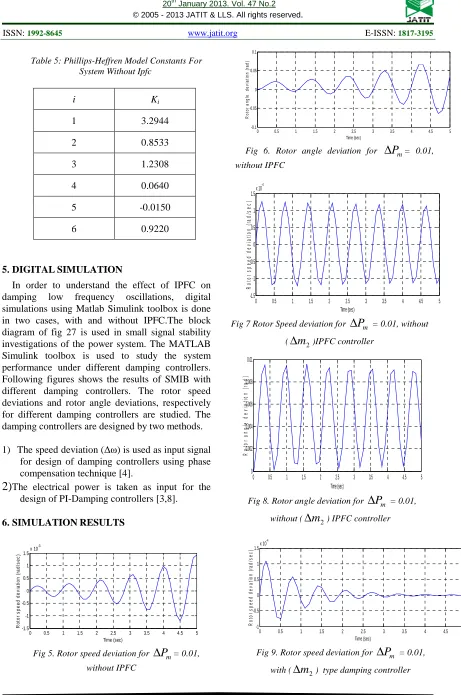
Table 5: Phillips-Heffren Model Constants For System Without Ipfc

i Ki

1 3.2944

2 0.8533

3 1.2308

4 0.0640

5 -0.0150

6 0.9220

5.DIGITALSIMULATION

In order to understand the effect of IPFC on damping low frequency oscillations, digital simulations using Matlab Simulink toolbox is done in two cases, with and without IPFC.The block diagram of fig 27 is used in small signal stability investigations of the power system. The MATLAB Simulink toolbox is used to study the system performance under different damping controllers. Following figures shows the results of SMIB with different damping controllers. The rotor speed deviations and rotor angle deviations, respectively for different damping controllers are studied. The damping controllers are designed by two methods.

1) The speed deviation (∆ω) is used as input signal for design of damping controllers using phase compensation technique [4].

2)

The electrical power is taken as input for the design of PI-Damping controllers [3,8].

6.SIMULATIONRESULTS

0 0.5 1 1.5 2 2.5 3 3.5 4 4.5 5

-1.5 -1 -0.5 0 0.5 1 1.5x 10

-3

Time (sec)

R

o

to

r

s

p

e

e

d

d

e

v

ia

ti

o

n

(

ra

d

/s

e

c

)

Fig 5. Rotor speed deviation for

∆

P

_m= 0.01, without IPFC

0 0.5 1 1.5 2 2.5 3 3.5 4 4.5 5

-0.1 -0.05 0 0.05 0.1

Time (sec)

R

o

to

r

a

n

g

le

d

e

v

ia

ti

o

n

(

ra

d

)

Fig 6. Rotor angle deviation for

∆

P

_m= 0.01, without IPFC

0 0.5 1 1.5 2 2.5 3 3.5 4 4.5 5 -1.5

-1 -0.5 0 0.5 1 1.5x 10

-4

Time (sec)

R

o

to

r

s

p

e

e

d

d

e

v

ia

ti

o

n

(

ra

d

/s

e

c

)

Fig 7 Rotor Speed deviation for

∆

P

_m = 0.01, without (

∆

m

₂)IPFC controller

0 0.5 1 1.5 2 2.5 3 3.5 4 4.5 5 0

0.002 0.004 0.006 0.008 0.01

Time (sec)

R

o

to

r

a

n

g

le

d

e

v

ia

ti

o

n

(

ra

d

)

Fig 8. Rotor angle deviation for

∆

P

_m = 0.01, without (

∆

m

₂) IPFC controller

0 0.5 1 1.5 2 2.5 3 3.5 4 4.5 5

-1 -0.5 0 0.5 1 1.5x 10

-4

Time (sec)

R

o

to

r

s

p

e

e

d

d

e

v

a

ti

o

n

(

ra

d

/s

e

c

)

[image:7.612.121.285.118.299.2]

0 0.5 1 1.5 2 2.5 3 3.5 4 4.5 5 0 0.002 0.004 0.006 0.008 0.01 Time (sec) R o to r a n g le d e v ia ti o n ( ra d )

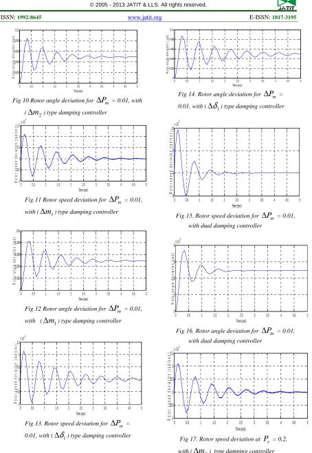
Fig 10 Rotor angle deviation for

∆

P

_m = 0.01, with (

∆

m

₂) type damping controller

0 0.5 1 1.5 2 2.5 3 3.5 4 4.5 5 -1

-0.5 0 0.5 1 1.5x 10

-4 Time (sec) R o to r s p e e d d e v ia ti o n ( ra d /s e c )

Fig 11 Rotor speed deviation for

∆

P

_m = 0.01,

with (

∆

m

₁) type damping controller

0 0.5 1 1.5 2 2.5 3 3.5 4 4.5 5

[image:8.612.90.544.57.716.2]

0 0.002 0.004 0.006 0.008 0.01 Time (sec) R o to r a n g le d e v ia ti o n ( ra d )

Fig 12 Rotor angle deviation for

∆

P

_m = 0.01, with (

∆

m

₁) type damping controller

0 0.5 1 1.5 2 2.5 3 3.5 4 4.5 5 -1

-0.5 0 0.5 1 1.5x 10

-4 Time (sec) R o to r s p e e d d e v ia ti o n ( ra d /s e c )

Fig 13. Rotor speed deviation for

∆

P

_m = 0.01, with (

∆

δ

₁) type damping controller

0 0.5 1 1.5 2 2.5 3 3.5 4 4.5 5

0 0.002 0.004 0.006 0.008 0.01 Time (sec) R o to r a n g le d e v ia ti o n ( r a d )

Fig 14. Rotor angle deviation for

∆

P

_m = 0.01, with (

∆

δ

₁) type damping controller

0 0.5 1 1.5 2 2.5 3 3.5 4 4.5 5 -5

0 5 10x 10

-5 Time (sec) R o to r s p e e d d e v ia ti o n ( ra d /s e c )

Fig 15. Rotor speed deviation for

∆

P

_m = 0.01, with dual damping controller

0 0.5 1 1.5 2 2.5 3 3.5 4 4.5 5 0

2 4 6 8x 10

-3 Time (sec) R o to r a n g le d e v ia ti o n ( ra d )

Fig 16. Rotor angle deviation for

∆

P

_m = 0.01, with dual damping controller

0 0.5 1 1.5 2 2.5 3 3.5 4 4.5 5 -1

-0.5 0 0.5 1 1.5x 10

-4 Time (sec) R o to r s p e e d d e v ia ti o n ( ra d /s e c )

[image:8.612.108.305.390.505.2]

ISSN: 1992-8645 www.jatit.org E-ISSN: 1817-3195

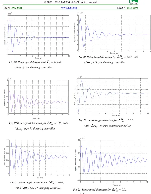
Fig 18. Rotor speed deviation at

P

_e = 1, with

(

∆

m

₂) type damping controller

Fig 19 Rotor speed deviation for

∆

P

_m = 0.01, with (

∆

m

₁) type PI-damping controller

Fig 20. Rotor angle deviation for

∆

P

_m = 0.01, with (

∆

m

₁) type PI- damping controller

Fig 21 Rotor Speed deviation for

∆

P

_m = 0.01, with (

∆

m

₂) PI type damping controller

Fig 22. Rotor angle deviation for

∆

P

_m = 0.01,

[image:9.612.79.563.57.678.2]

with (

∆

m

₂) PI type damping controller

[image:10.612.91.303.74.265.2] [image:10.612.89.303.261.595.2]

Fig 24 Rotor angle deviation for

∆

P

_m = 0.01, with(

∆

δ

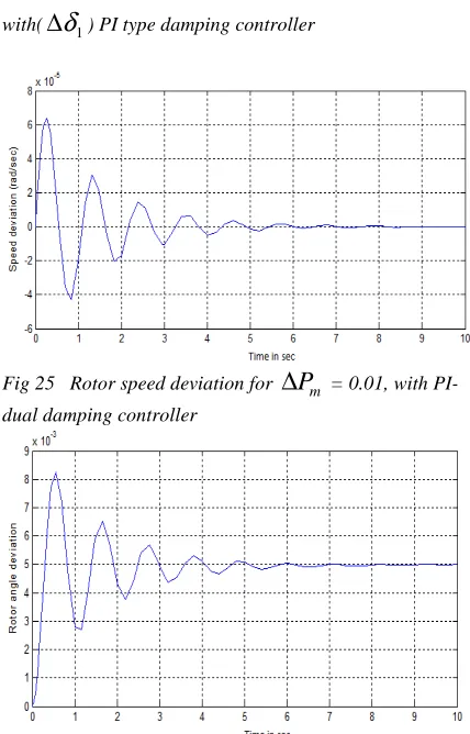
₁) PI type damping controller

Fig 25 Rotor speed deviation for

∆

P

_m = 0.01, with PI- dual damping controller

Fig 26 Rotor angle deviation for

∆

P

_m = 0.01, with PI- dual damping controller

7.CONCLUSIONS

The IPFC based damping controller is

designed for two different cases. The output of

the power system without IPFC, with IPFC are

obtained and compared.

IPFC as a multitask controller, has an

effective role in damping low frequency

oscillations. In this thesis, this function of

IPFC has been investigated and numerical

results emphasized its significant effect. In

fact, even there is not any damping coefficient

in power systems, IPFC can damp low

frequency oscillations. These effects are

decreasing the amplitude and frequency of

power system oscillations. Moreover it damps

oscillations faster in comparison when there is

not IPFC in the system. The controllability

index

corresponding

to

IPFC

control

parameter

∆

m

₂

, is highest and that of

∆

δ

₂

,

is insignificant compared to the other control

parameters. Hence,

∆

u =

∆

m

₂

is the best

selection for the design of the IPFC damping

controller since the minimum control cost (the

lowest gain) is needed to provide , the

damping controllers based on

∆

m

₂

_.

Dynamic simulations results have

emphasized that the damping controller which

modulates the control signal

∆

m

₂

provides

satisfactory dynamic Performance under wide

variations in loading condition and system

parameters.

The response of the SMIB installed with

IPFC based Dual converter is improved when

compared to without IPFC and individual

(

m

₁

,

δ

₁

,and

m

₂

) type damping controllers.

Response of SMIB with IPFC for step

perturbation in

∆

P

_m

= 0.01 ,and

∆

V

_ref

= 0.01

is good with Dual controller.

The settling time for PI- damping

controller is more as compared to

Phase-compensation based damping controllers.

Phase-compensation

based

damping

ISSN: 1992-8645 www.jatit.org E-ISSN: 1817-3195

Table 6: Comparison of Settling Time for Two cases

IPFC damping controller

PI Controller

Phase

Compensation

1

m

_{-type controller} 10 sec 4.5 sec

1

δ

_{-type controller} 10 sec 5 sec

2

m

_{-type controller} 9 sec 4 sec

Dual converter 8 sec 3 sec

APPENDIX

The system data and initial operating conditions of the system are as follows:

Generator:

M = 2H = 8.0 MJ/MVA

D = 0; Tdo = 5.044s;

X

_d=1.0pu;

X

'd = 0.3pu; q

X

= 0.6pu ;

P

_e= 0.900; Q = 0.1958 ;

V

_s = 1.02;

1

=

b

V

Excitation system:

K

A= 50;

T

_A = 0.05s

Converter transformers:

X

_t= 0.l pu

Converter parameters:

m

₁= 0.15;

m

₂=0.10; Transmission line transformers:

L

X

= 0.5 pu;

X

_s=0.15 pu

DC link parameters:

V

_dc= 2.0 pu; C = 1 pu

REFERENCES

[1] Yao-nan Yu, "ELECTRIC POWER SYSTEM DYNAMICS", New York, Academic Press, Inc. , 1983

[2] Guygyi & etal " THE INTERLINE POWER FLOW CONTROLLER CONCEPT: A NEW

APPROACH TO POWER FLOW

MANAGEMENT IN TRANSMISSION

SYSTEMS", IEEE Transactions on Power Delivery, Vol. 14, No. 3, July 1999.

[3] H.F.Hang, "DESIGN OF SSSC DAMPING

CONTROLLER TO IMPROVE POWER

SYSTEM OSCILLATION STABILITY",

19991EEE.

[4] N.Tambey and M.L.Kothari, "DAMPING OF POWER SYSTEM OSCILLATION WITH UNIFIED POWER FLOW CONTROLLER", IEE Proc.-Gener. Transm. Distrib. Vol.150, No.2, March 2003.

[5] "FLEXIBLE AC TRANSMISSION SYSTEMS (FACTS)", IEE Press, London 1999.

[6] K. V. Patil, J. Senthil, J. Jiang and R. M. Mathur, “Application of STATCOM for Damping Torsional Oscillations in Series Compensated AC Systems,” IEEE Transactions on Energy Conversion, vol. 13, No. 3, September 1998, pp. 237-243.

[7] H.F.Wang and F.J.Swift, “A Unified Model for the Analysis of FACTS Devices in Damping Power System Oscillations Part I: Single-Machine Infinite-bus Power

System,” IEEE Transactions on Power Delivery, vol. 12, No. 2, April 1997, pp. 941-946.

[image:12.612.95.483.129.458.2]