CRL 96 1 pdf

(1)

Shape Ambiguities in Structure from

Motion

Richard Szeliski and Sing Bing Kang

Digital Equipment Corporation

Cambridge Research Lab

(2)

Digital Equipment Corporation has four research facilities: the Systems Research Center and the Western Research Laboratory, both in Palo Alto, California; the Paris Research Laboratory, in Paris; and the Cambridge Research Laboratory, in Cambridge, Massachusetts.

The Cambridge laboratory became operational in 1988 and is located at One Kendall Square, near MIT. CRL engages in computing research to extend the state of the computing art in areas likely to be important to Digital and its customers in future years. CRL’s main focus is applications technology; that is, the creation of knowledge and tools useful for the preparation of important classes of applications.

CRL Technical Reports can be ordered by electronic mail. To receive instructions, send a mes-sage to one of the following addresses, with the word help in the Subject line:

On Digital’s EASYnet: CRL::TECHREPORTS

On the Internet: [email protected]

This work may not be copied or reproduced for any commercial purpose. Permission to copy without payment is granted for non-profit educational and research purposes provided all such copies include a notice that such copy-ing is by permission of the Cambridge Research Lab of Digital Equipment Corporation, an acknowledgment of the authors to the work, and all applicable portions of the copyright notice.

The Digital logo is a trademark of Digital Equipment Corporation.

Cambridge Research Laboratory One Kendall Square

Cambridge, Massachusetts 02139

(3)

Shape Ambiguities in Structure from

Motion

Richard Szeliski

1

and Sing Bing Kang

Digital Equipment Corporation

Cambridge Research Lab

CRL 96/1 February, 1996

Abstract

This technical report examines the fundamental ambiguities and uncertainties inherent in

recov-ering structure from motion. By examining the eigenvectors associated with null or small

eigen-values of the Hessian matrix, we can quantify the exact nature of these ambiguities and predict how

they affect the accuracy of the reconstructed shape. Our results for orthographic cameras show that

the bas-relief ambiguity is significant even with many images, unless a large amount of rotation

is present. Similar results for perspective cameras suggest that three or more frames and a large

amount of rotation are required for metrically accurate reconstruction.

Keywords: Structure from motion, ambiguities, uncertainty analysis

(4)

(5)

Contents i

6 Orthography: full 3-D reconstruction : : : : : : : : : : : : : : : : : : : : : : : : : 17 7 Perspective: single scanline : : : : : : : : : : : : : : : : : : : : : : : : : : : : : : 19 8 Perspective in 3-D : : : : : : : : : : : : : : : : : : : : : : : : : : : : : : : : : : : 21 8.1 Pure object-centered rotations . . . 21

8.2 Looming . . . 24

9 Experimental results : : : : : : : : : : : : : : : : : : : : : : : : : : : : : : : : : : 25 10 Discussion : : : : : : : : : : : : : : : : : : : : : : : : : : : : : : : : : : : : : : : : 27 10.1 Future work . . . 28

11 Conclusions : : : : : : : : : : : : : : : : : : : : : : : : : : : : : : : : : : : : : : : 29

(6)

ii LIST OF TABLES

List of Figures

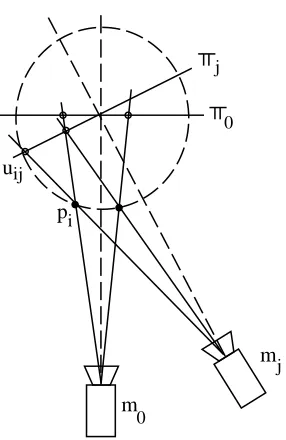
1 Sample configuration of cameras (

m

j), 3-D points (

p

i), image planes( j), and screen

locations (

u

ij) . . . 5

2 Constraint lines and energy surface for simple two-parameter example. Thex-axis

is the angleand they-axis is the scale factora. . . 9

3 Orthographic projection, two frames. . . 12

4 Plot oflog10min as a function ofJ 218]and20:11:5]. . . 15

5 Minimum eigenvector for a three-frame perspective reconstruction problem: (a)

top-down view (x-z), (b) frontal view (x-y). While the main ambiguity is az

scal-ing, the vector is not exactly an affine transform of the 3-D points on the unit cube. 24

6 Minimum eigenvector for a three-frame perspective reconstruction problem with

pureztranslation: (a) top-down view (x-z), (b) frontal view (x-y). The main

am-biguity is a rocking confusion between sideways camera translation and rotation,

which affects the points furthest back. . . 26

List of Tables

1 Minimum eigenvalues for 1-D orthographic known equi-angular motion . . . 15

2 Minimum eigenvalues for 1-D orthographic equi-angular motion with no constraint 16

3 S

allestimates for 1-D orthographic equi-angular motion with no constraint, X =

Z =100,=1. . . 17

4 Minimum eigenvalues for 2-D orthographic equi-angular motion with no constraint,

rotation aroundyaxis (q1 =sin

j

2 ,q2 =0). . . 19

5 Minimum eigenvalues for 2-D orthographic equi-angular motion with no constraint,

rotation aroundyaxis tilted30 (q1 =cos30 sin

j

2 ,q2 =sin30 sin

j

2 ). . . 19 6 Minimum eigenvalues for 1-D perspective projection, equi-angular rotation,=0:2. 20

7 Minimum eigenvalues for 3-D perspective projection, equi-angular rotation around

yaxis,=0:1. . . 21

(7)

LIST OF TABLES iii

yaxis, three frames (F =3), varying. is the camera’s field of view. . . 23

10 RMS

posfor 3-D perspective projection, equi-angular rotation around

yaxis,=0:1. 23

11 Minimum eigenvalues for 3-D perspective projection, pure forward translation,=

0:3. . . 25

12 Minimum eigenvalues for 3-D perspective projection, pure forward translation,F =

2, varying. . . 25

13 RMS errors (predicted and observed) for 3-D perspective projection, equi-angular

rotation aroundyaxis, two frames, 24 point data set. . . 27

14 RMS errors (predicted and observed) for 3-D perspective projection, equi-angular

(8)

(9)

1 Introduction 1

1 Introduction

Structure from motion is one of the classic problems in computer vision and has received a great

deal of attention over the last decade. It has wide-ranging applications, including robot vehicle

guidance and obstacle avoidance, and the reconstruction of 3-D models from imagery.

Unfortu-nately, the quality of results available using this approach is still often very disappointing. More

precisely, while the qualitative estimates of structure and motion look reasonable, the actual

quan-titative (metric) estimates can be significantly distorted.

Much progress has been made recently in identifying the sources of errors and instabilities in

the structure from motion process. It is now widely understood that the arbitrary algebraic

manip-ulation of the imaging equations to derive closed-form solutions (e.g., [LH81]) can lead to

algo-rithms that are numerically ill-conditioned or unstable in the presence of measurement errors. To

overcome this, statistically optimal algorithms for estimating structure and motion have been

devel-oped [SA89; WAH89; Hor90; TK92b; SK94]. It is also understood that using more feature points

and images results in better estimates, and that certain configurations of points (at least in the two

frame case) are pathological and cannot be reconstructed.

An example of an algorithm which generates very good results is the factorization approach of

Tomasi and Kanade [TK92b]. This algorithm assumes orthography and is implemented using an

object-centered representation and singular value decomposition. It uses many points and frames,

and for most sequences, a large amount of object rotation (usually360 ). However, when only a

small range of viewpoints is present (e.g., the “House” sequence in [TK92b], Figure 7), the

recon-struction no longer appears metric (the house walls are not perpendicular).

In this technical report, we demonstrate that it is precisely this last factor, i.e., the overall

ro-tation of the object, or equivalently, the variation in viewpoints, which critically determines the

quality of the reconstruction. The ambiguity in object shape due to small viewpoint variation

of-ten looks like it might be a projective deformation of the Euclidean shape, which is interesting—

several researchers have argued recently in favor of trying to recover only this projective structure

[Fau92; HGC92; MQVB92; Sha93]. In fact, we show that the major ambiguity in the reconstruction

is a simple depth scale uncertainty, i.e., the classic bas-relief ambiguity which exists for two-frame

structure from motion under orthographic projection [LH86].1

1

(10)

2 2 Previous work

To derive our results, we use eigenvalue analysis of the covariance matrix for the structure and

motion estimates. This assumes that we can compute a near optimal solution, and that the error in

the solution is due to linear perturbations arising from small amounts of image noise (feature point

mislocalization). This kind of analysis has not previously been applied to structure from motion,

and yet it is a very powerful way to predict the ultimate performance of structure from motion

al-gorithms.

Our results are significant for two reasons. First, we show how to theoretically derive the

ex-pected ambiguity in a reconstruction, and also derive some intuitive guidelines for selecting

imag-ing situations which can be expected to produce reasonable results. Second, since the primary

am-biguities are very well characterized by a small number of modes, this information can be used to

construct better on-line (recursive) estimation algorithms.

Our technical report is structured as follows. After reviewing previous work, we present our

formulation of the structure from motion problem and develop our technique for analyzing

ambi-guities using eigenvector analysis of the information (Hessian) matrix. We then present the results

of our analysis for a series of camera models: 1-D and 2-D orthographic cameras, and 1-D and 2-D

perspective cameras. We conclude with a discussion of the main sources of errors and ambiguities,

and directions for possible future work.

2 Previous work

Structure from motion has been extensively studied in computer vision. Early papers on this

sub-ject [LH81; TH84] develop algorithms to compute the structure and motion from a small set of

points matched in two frames using an essential parameter approach. The performance of this

ap-proach can be significantly improved using non-linear least squares (optimal estimation) techniques

[WAH89; WAH93; SA89; Hor90; SA91].

Recent research focuses on extraction of shape and motion from longer image sequences [KTJ89;

DA90; CWC90; TK92b; CT92]. Cui, Weng, and Cohen [CWC90] use an optimal estimation

tech-nique (non-linear least squares) between each pair of frames, and an extended Kalman filter to

accu-mulate information over time (see also [THO93; SPFP93]). Azarbayejani et al. [AHP93] also use a

Kalman filter-based approach to recover rigid (object-centered) depth and motion directly from the

sequence of image measurements. Tomasi and Kanade [TK92b] use a factorization method which

(11)

3 Problem formulation and uncertainty analysis 3

approach formulates the shape from motion problem in object-centered coordinates, assumes

or-thography, and processes all of the frames simultaneously. Chen and Tsuji [CT92] relax the

as-sumption of orthography by analyzing the image sequence through its temporal and spatial subparts.

Taylor and Kriegman [TKA91; TK92a] formulate the shape from motion task as a non-linear least

squares problem in which the Euclidean distance between the estimated and actual positions of the

points in the image sequence is minimized using the Levenberg-Marquardt algorithm. Szeliski and

Kang [SK94] extend this approach approaches to general 3-D structure and also to projective

struc-ture and motion recovery.

Another line of research has addressed recovering affine [KvD91; SZB93] or projective [Fau92;

HGC92; HG93; MVQ93] structure estimates. Most of these techniques rely on identifying and

tracking a small number of feature points in the image sequence, using these points to form a basis

set for the geometric description, and also only use 2 frames to recover the geometry. However,

Mohr et al. [MVQ93] and Szeliski and Kang [SK94] use as many points and frames as possible to

recover the geometry and motion, thus producing more reliable estimates.

The nature of structure and motion errors, which is the main focus of this technical report, has

also previously been studied. Weng et al. perform some of the earliest and most detailed error

anal-yses of the two-frame essential parameter approach [WAH89; WAH93]. Adiv [Adi89] and Young

and Chellappa [YC92] analyze continuous-time (optical flow) based algorithms using the concept

of the Cramer-Rao lower bound. Oliensis and Thomas [OT91; THO93] show how modeling the

motion error can significantly improve the performance of recursive algorithms.

In this technical report, we extend these previous results using an eigenvalue analysis of the

covariance matrix. This analysis can pinpoint the exact nature of structure from motion ambiguities

and the largest sources of reconstruction error. We also focus on multi-frame optimal structure from

motion algorithms, which have not been studied in great detail.

3 Problem formulation and uncertainty analysis

Structure from motion can be formulated as the recovery of a set of 3-D structure parameters

p

i

and time-varying motion parameters

m

jfrom a set of observed image features

u

ij. In this section,

we present the forward equations, i.e., the rigid body and perspective transformations which map

3-D points into 2-D image points. We also show how the Jacobians of the forward equation can

(12)

4 3 Problem formulation and uncertainty analysis

be used to quantify expected reconstruction errors, and how our results relate to classical structure

from motion ambiguities.

3.1 Problem formulation

The equation which projects theith 3-D point

p

i into the

jth frame at location

u

ij is

u

ij

=P(T(

p

i

m

j

)): (1)

The perspective projectionP (defined below) is applied to a rigid transformation

T(

p

i

m

j

)=

R

j

p

i

+

t

j

(2)

where

R

jis a rotation matrix and

t

jis a translation applied after the rotation. A variety of alternative

representations are possible for the rotation matrix [Aya91]. In this technical report, we primarily

use a quaternion

q

=w (q0q1q2)]representation, with a corresponding rotation matrix

R

(

q

)= 0 B B B @

1;2q21;2q22 2q0q1+2w q2 2q0q2;2w q1 2q0q1;2w q2 1;2q20;2q22 2q1q2+2w q0 2q0q2+2w q1 2q1q2 ;2w q0 1;2q20;2q21

1 C C C A (3)

since this representation has no singularities. The rotation parametersq0q1q2 also have a natural

interpretation (for small values) as the half-angles of rotation around thex,y, andz axes. For our

one-dimensional examples, we use the rotation angle around the vertical axis.

The standard perspective projection equation used in computer vision is

0 @ u v 1 A

=P1 0 B B B @ x y z 1 C C C A 0 @ f x z f y z 1 A (4)

wherefis a product of the focal length of the camera and the pixel scale factor (assuming that pixels

are square). An alternative object-centered formulation, which we introduced in [SK94] is

0 @ u v 1 A

(13)

3.1 Problem formulation 5

u_ij

i p

m j m

0

[image:13.612.237.380.102.322.2]

0 j

Figure 1: Sample configuration of cameras (

m

j), 3-D points (

p

i), image planes( j), and screen

locations (

u

ij)

Here, we assume that the(xyz)coordinates before projection are with respect to a reference frame

j that has been displaced away from the camera by a distance t

z along the optical axis, with s = f=t

zand

=1=t

z (Figure 1). The projection parameter

scan be interpreted as a scale factor and

as a perspective distortion factor. Our alternative perspective formulation allows us to model both

orthographic and perspective cameras using the same model.

A variety of techniques (reviewed in Section 2) can be used to estimate the unknownsf

p

i

m

j

g

from the given image measurements f

u

ij

g. In our previous work [SK94], we used the iterative

Levenberg-Marquardt algorithm, since it provides a statistically optimal solution [WAH89; SA89;

TK92a; SK94]. The Levenberg-Marquardt method is a standard non-linear least squares technique

[PFTV92] which directly minimizes a merit or objective function

C(

a

)= X

i X

j c

ij j~

u

ij ;

f

ij (

a

)j

2

(6)

where

u

~

ij is the observed image measurement,

f

ij

(

a

) =

u

(

p

i

m

j

)is given in (1), and the vector

a

contains all of the unknown structure and motion parameters, including the 3-D points

p

i, the

motion parameters

m

j, and any additional unknown calibration parameters. The weight c

ij in (6)

describes the confidence in measurement

u

ij, and is normally set to the inverse variance

(14)

6 3 Problem formulation and uncertainty analysis

be set to zero for missing measurements).

3.2 Uncertainty analysis

Regardless of the solution technique, the uncertainty in the recovered parameters—assuming that

image measurements are corrupted by small Gaussian noise errors—can be determined by

comput-ing the inverse covariance or information matrix

A

[Sor80]. This matrix is formed by computing outer products of the Jacobians of the measurement equations

A

= X i X j c ij @

f

T ij @

a

@

f

ij @

a

T : (7)

For notational succinctness, we use the symbol

H

ij = 2 6 4 @

f

T ij @

p

i @

f

T ij @

m

j 3 7 5

to denote the non-zero portion of the full Jacobian @

f

T ij @

a

.

If we list the structure parametersf

p

i

gfirst, followed by the motion parametersf

m

j

g, the

A

matrix has the structure

A

= 2

4

A

p

A

pm

A

T

pm

A

m

3 5

: (8)

The matrices

A

p

and

A

m

are block diagonal, with diagonal entries

A

p

i = X j @

f

T ij @

p

i @

f

ij @

p

T i

and

A

m

j = X i @

f

T ij @

m

j @

f

ij @

m

T j (9)

respectively (assumingc ij

=1), while

A

pm

is dense, with entries

A

p

i

m

j = @

f

T ij @

p

i @

f

ij @

m

T j : (10)

The information matrix has previously been used in the context of structure from motion to

de-termine Cramer-Rao lower bounds on the parameter uncertainties by taking the inverse of the

diag-onal entries [Adi89; YC92]. The Cramer-Rao bounds, however, can be arbitrarily weak, especially

when

A

is singular or near-singular. In this technical report, we use eigenvector analysis of

A

to find the dominant directions in the uncertainty (covariance) matrix and their magnitudes, which

(15)

3.3 Estimating reconstruction errors 7

3.3 Estimating reconstruction errors

An important benefit of uncertainty analysis is that we can easily quantify the expected amount of

reconstruction (and motion) error for an optimal structure from motion algorithm. For example, the

expected sum of squared error in reconstructed 3-D point positions is

S

2

pos

* X

i k

p

~

i ;

p

i k

2

+

(11)

where

p

~

i are the estimated (recovered) positions and

p

i the true positions. The positional

uncer-tainty matrix

C

p

can be computed by inverting

A

and looking at its upper left block (the block corresponding to the

p

i variables).2 If we perform an eigenvalue analysis of

C

p

, we obtain

C

p

=

E

T

p p

E

p

(12)

where

E

p

is the matrix of eigenvectors, and

p

is the diagonal matrix containing the eigenvalues of

C

p

. SinceS2

pos

is a Euclidean norm, its value is unaffected by orthogonal coordinate

transfor-mations such as

E

p

. The value ofS2 pos

can thus be computed as either the trace of

C

p

or the trace of

p

, i.e., the sum of the eigenvalues of

C

p

.

In practice, we do not need to compute

C

p

. Instead, the sum of squared reconstruction and motion error,

S

2

all

* X

i k

p

~

i ;

p

i k

2

+ X

j k

m

~

j ;

m

j k

2

+

(13)

can be computed directly summing the inverse eigenvalues of the information matrix

A

. By choos-ing an appropriate scalchoos-ing for the parameters bechoos-ing estimated (say scalchoos-ing positions to be in the

range;100:::100]and rotations in the range; ::: ]), we can make the mean ofS

allbe close

to the mean ofS

pos. Note that for general 3-D camera motion, positional errors in the motion

esti-mates will be on the same scale as 3-D reconstruction errors, and may sometimes dominate (if the

absolute distance of the camera is ill determined).

What is the advantage of this approach, if computing eigenvalues is just as expensive as

invert-ing matrices? First, we can compute the first few eigenvalues more cheaply (and in less space) than

the matrix inverse, and these tend to dominate the overall reconstruction error. Second, it justifies

the approach in the technical report, which is to look at the minimum eigenvalue as the prime

in-dicator of reconstruction error. We can therefore study how much certain ambiguities (such as the

2

(16)

8 4 A two parameter example

bas-relief ambiguity) contribute to the overall reconstruction error. We can also obtain much tighter

lower bounds on the reconstruction error than would be possible by using the Cramer-Rao bounds.

3.4 Ambiguities in structure from motion

Because structure from motion attempts to recover both the structure of the world and the camera

motion without any external (prior) knowledge, it is subject to certain ambiguities. The most

fun-damental (but most innocuous) of these is the coordinate frame (also known as pose, or Euclidean)

ambiguity, i.e., we can move the origin of the coordinate system to an arbitrary place and pose and

still obtain an equally valid solution.

The next most common ambiguity is the scale ambiguity (for a perspective camera) or the depth

ambiguity (for an orthographic camera). This ambiguity can be removed with a small amount of

additional knowledge, e.g., the absolute distance between camera positions.

A third ambiguity, and the one we focus on in this technical report, is the bas-relief ambiguity.

In its pure form, this ambiguity occurs for a two frame problem with an orthographic camera, and

is a confusion between the relative depth of the object and the amount of object rotation. In this

technical report, we focus on the weak form of this ambiguity, i.e., the very large bas-relief

uncer-tainty which occurs with imperfect measurements even when we use more than two frames and/or

perspective cameras. A central result of this technical report is that the bas-relief ambiguity

cap-tures the largest uncertainties arising in structure from motion. However, when examined in detail,

it appears that a larger class of deformations (i.e., projective) more fully characterizes the errors

which occur in structure from motion.

To characterize these ambiguities, we will use eigenvector analysis of the information matrix,

as explained in Section 3.2. Absolute ambiguities will show up as zero eigenvalues (unless we add

additional constraints or knowledge to remove them), whereas weak ambiguities will show up as

small eigenvalues.

4 A two parameter example

To develop an intuitive understanding of the basic bas-relief ambiguity, we start with a simple

two-parameter example. Assume that we have an orthographic scanline camera which measures thex

(17)

4 A two parameter example 9

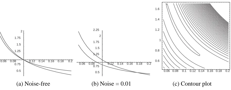
0.06 0.08 0.12 0.14 0.16 0.18 0.2 0.5 0.75 1.25 1.5 1.75 2

0.06 0.08 0.12 0.14 0.16 0.18 0.2 0.5 0.75 1.25 1.5 1.75 2 2.25

0.06 0.08 0.1 0.12 0.14 0.16 0.18 0.2 0.6 0.8 1 1.2 1.4 1.6

[image:17.612.79.536.108.287.2]

(a) Noise-free (b) Noise = 0.01 (c) Contour plot

Figure 2: Constraint lines and energy surface for simple two-parameter example. Thex-axis is the

angleand they-axis is the scale factora.

factor in depth,

p

i =(x i az i )

and that the rotation angles are uniform,

j

=j :

The projection equation is then

u ij =c j x i ;s j az i (14) withc j =cos j and s j =sin j.

What happens when we try to estimate the scale factoraand the anglefrom a set of noisy

measurements fu ij

g? First, let’s examine the very simplest case, which is a single point, say at (xz)=(11). Each new image gives us a constraint of the form

c j ;as j =c j ;a s j +n j (15) wherec j, s j, and

a

are the true values andn

jis random noise. Figure 2a shows the two constraint

lines forj = 1assuming the noise-free case (witha = 1and = 0:1rad). Figure 2b shows

the constraint lines forn ;1

=n1 =0:01. As can be seen, the estimate for( a)is very sensitive

to noise. This can also be seen in the contour plot of the energy surface (Figure 2c) which can be

(18)

10 5 Orthography: single scanline

To characterize the shape of the error surface near its minimum, we compute the information

matrix

A

. The Jacobian for(a )is straightforward,

H

ij = 2 4 @u ij @a @u ij @ 3 5 = 2 4 ;s j z i ;j(ac j z i +s j x i ) 3 5 ;j 2 4 z i az i

+j x i

3

5 (16)

if we assume small rotation angles,j j

j1, so thats j

jandc j

1. The inverse covariance

(information) matrix is then

A

J2Z 2 4

2 a

a a2+2 J 4 X J 2 Z 3 5 (17)

whereJ2 = P

j

j2,J4 = P

j

j4,X = P

i x

2

i, and Z =

P i

z

2

i (assuming that P

j

j =0). Assuming

that

2

a2, we can compute (Appendix A) the approximate eigenvalues of

A

as min

4

J4X=a

2 _and

maxJ2Za

2

: (18)

The eigenvalues of the information matrix describe an “elliptic” approximation to the error

sur-face (and hence posterior probability distribution), which matches the true “banana shaped” sursur-face

near the optimal solution but not far away from it. To determine if the additional nonlinearities in

the reconstruction process result lower or higher overall uncertainties than those predicted by the

information matrix, we would have to resort to numerical simulations. In practice, we expect these

secondary effect to be much smaller than the large variations in eigenvalues which explain most of

the uncertainties (ambiguities) associated with structure from motion.

5 Orthography: single scanline

Let us now turn to a true structure from motion problem where both the structure and motion are

unknown. For simplicity, we analyze the orthographic scanline camera first, where the unknowns

are the 2-D point positions

p

i =(x

i z

i

)and the rotation angles

j.3 The imaging equations are

u ij =c j x i ;s j z i (19) withc j =cos j and s j =sin j. 3

(19)

5.1 Two frames: the bas-relief ambiguity 11

The Jacobian for the 1-D orthographic camera is

H

ij = h @uij @xi @uij @zi @uij @j i T = h c j ;s j ;(c j z i +s j x i ) i T (20)

and the entries in the information matrix are

A

p

i = 2 4 P j c2 j ; P j c j s j ; P j c j s j P j s2 j 3 5 = 2 4 C ;D ;D S 3 5 (21)

A

p

i

m

j = 2 4 ;c 2 j z i ;c j s j x i c j s j z i +s 2 j x i 3 5 (22)

A

m

j = h P i (c j z i +s j x i ) 2 i = h c 2 j

Z+2c j

s j

W+s

2

j X

i

(23)

withC = P

j c2

j

,D = P j c j s j, S = P j s2 j

,Z = P

i z2

i

,W = P

i z

i x

i, and X = P i z2 i .

Before analyzing the complete information matrix, let us look at the two subblocks

A

p

and

A

m

. If we know the motion, the structure uncertainty is determined by

A

p

i

and is simply the

triangula-tion error, i.e.,2 x

/C ;1 and

2 z

/S

;1 (note that for small rotations, 2

x

is generally much smaller

than

2

z). If we know the structure, the motion accuracy is determined by

A

m

j and is inversely

proportional to the variance in depth along the viewing direction(s j

c j

).

What about ambiguities in the solution? Under orthography, the traditional scale ambiguity does

not exist. However, translations along the optical axis cannot be estimated, and an overall pose

(coordinate frame) ambiguity still exists. Unless we add some additional constraints, we can always

rotate the coordinate system by aand add the same amount to thef j

g. This manifests itself as

the null (zero eigenvalue) eigenvector

e

0 = h

z0 ;x0 z N

;x N

1 1 i

T :

5.1 Two frames: the bas-relief ambiguity

Let us say we only have two frames, and we have fixed0 =0c0 =1s0=01 = c1 =cs1 =

s(Figure 3). Then

A

p

i =

2 4

1+c2 ;cs ;cs s2

3

5 (24)

A

p

i

m

= 2 4 ;c 2 z i ;csx i csz i +s2x

i 3

5 (25)

A

m

= h

c2Z+2csW +s2X i

(20)

x z

z

δ

δθ θ

x z

z δ

δθ x

δ

δθ

θ θ

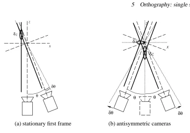
[image:20.612.115.503.71.343.2]

(a) stationary first frame (b) antisymmetric cameras

Figure 3: Orthographic projection, two frames.

The solid lines indicate the viewing rays, while the thin lines indicate the optical axes and image

planes. The diagonal dashed lines are the displaced viewing rays, while the ellipses indicate the

positional uncertainty in the reconstruction due to uncertainty in motion (indicated as).

The bas-relief ambiguity manifests itself as a null eigenvector

e

0= h

0 cz0+sx0 0 cz N

+sx N

;s i

T

as can be verified by inspection. This is as we expected, i.e., the primary uncertainty in the structure

is entirely in the depth (z) direction, and is a scale uncertainty (proportional toz). Note however

that this uncertainty is proportional tocz+sxrather thanz, as can be seen by inspecting Figure 3a.

An alternative parameterization of the two-frame problem is to set 0 = ;1 (Figure 3b), in

which case we have

A

p

i =

2 4

2c2 0 0 2s2

3

5 (27)

A

p

i

m

=

2 4

;2csx i 2csz

i 3

5 (28)

A

m

= h

2c2Z+2s2X i

(21)

5.2 More than two frames, equi-angular motion constraint 13

In this case, the null eigenvector is

e

0 = h

s

2

x0 ;c

2 z i s 2 x N ;c 2 z N cs i T : (30)

This is also very illuminating. It shows that the primary effect of the bas-relief ambiguity is a

“squashing” of thezvalues for a small increase in motion, with a much smaller “bulging” in thex

values (at least for small inter-frame rotations).4 This squashing and bulging is an affine

deforma-tion of the true structure.

5.2 More than two frames, equi-angular motion constraint

To simplify the analysis, we assume for the moment that we know we have an equi-angular image

sequence, i.e., that the rotation angles are given by j

=j,j 2 f;J:::Jg,J = F+1

2 , where

F is the total number of frames (imagine Figure 3b with more cameras). In this case, we have

H

T ij = h c j ;s j ;j(c j z i +s j x i ) i (31)

A

p

i = 2 4 P j c 2 j 0 0 P j s 2 j 3 5 = 2 4 C 0 0 S 3 5 (32)

A

p

i

m

= 2 4 ; P j jc j s j x i P j jc j s j z i 3 5 = 2 4 ;Ex i Ez i 3 5 (33)

A

m

= h

P j

j2c2 j

Z+ P

j j2s2

j X i = h C 0 Z +S

0 X

i

(34)

withE = P j jc j s j, C 0 = P j

j2c2 j, S 0 = P j j2s2

j, and

C D SZ WX defined as in (22–23). In

this case, the smallest eigenvalue eigenvector has the form

e

0 = h

x0 ;z0 x N ;z N 1 i T : (35)

This will be an eigenvector if we can satisfy the matrix equation

Ae

=

e

, i.e.,

2

4

A

p

A

pm

A

T

pm

A

m

3 5 2 6 6 6 6 6 6 6 6 6 4 x0 ;z0 .. . ;z N 1 3 7 7 7 7 7 7 7 7 7 5 = 2 6 6 6 6 6 6 6 6 6 4 x0 ;z0 .. . ;z N 1 3 7 7 7 7 7 7 7 7 7 5 4

(22)

which reduces to the following three equations:

C;E =

S;E =

(S 0

;E)X +(C 0

;E)Z = :

Substituting= E C;

and = E S;

into the third equation, we obtain a cubic in,

(S;)(S 0

(C;);E

2

)X+(C ;)(C 0

(S;);E

2

)Z;(S;)(C;) =0 (36)

which can be solved analytically using a package such as MathematicaR [Wol91].

Assuming that the smallest eigenvalue is very small, we can use the approximation E C

to

obtain a quadratic in,

(S;)(S 0

C;E

2

)X +C(C 0

(S;);E

2

)Z;(S;)C=0: (37)

Furthermore, using the small angle approximations, C P

j

1 J0,S 2J2,E J2, C

0

J2, andS 0

2J4, we obtain after some manipulation (Appendix A)

min

4XJ2(J0J4;J22)

J0J2Z +2X(J0J4;J22)+J0J2]

: (38)

Notice that the minimum eigenvalue is related to the fourth power of, i.e., doubling the

inter-frame rotation reduces the RMS (root mean square) error by a factor of 4 (assuming thatZ 2).

Increasing the extent of thex

i compared to the z

i directly increases the minimum eigenvalue, i.e.,

it decreases the structure uncertainty. This result is somewhat surprising, and suggests that flatter

objects can be reconstructed better.

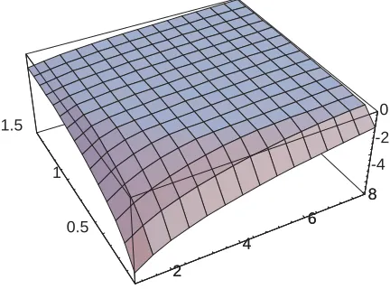
We can numerically compute the values offor a range ofJ andvalues (Figure 4). For

ex-ample, withJ =1, =0:1rad6 , andX =Z =1, we have=f0:0000664436 1:980 643 :0193 g.

For the smallest eigenvalue, = 0:0000664436, we have a corresponding = 0:0666676 and

=10:0001.

Once the smallest eigenvalue and eigenvector have been computed, we can easily determine

some additional eigenvectors. Any vector which consists purely ofx i or

z

i values which is also

orthogonal to

A

pm

is an eigenvector, e.g.,

e

= h

x1 0 ;x0 0 0 0 i

(23)

5.2 More than two frames, equi-angular motion constraint 15

2

4

6 8

0.5 1 1.5

-4 -2

0

2

4

[image:23.612.196.412.121.281.2]

6 8

Figure 4: Plot oflog10min as a function ofJ 218]and 20:11:5].

min F =2 F =3 F =4 F =5 F =6 F =7 F =8

tot=11:5 0:000000 0:000067 0:000079 0:000088 0:000096 0:000104 0:000112 tot=22:9 0:000000 0:001087 0:001283 0:001418 0:001547 0:001677 0:001810 tot=34:4 0:000000 0:005618 0:006597 0:007277 0:007931 0:008594 0:009269 tot=45 0:000000 0:016854 0:019688 0:021673 0:023596 0:025552 0:027547 tot=60 0:000000 0:054679 0:063442 0:069678 0:075782 0:082017 0:088389 tot=90 0:000000 0:272977 0:316453 0:348500 0:380039 0:412200 0:444997

Table 1: Minimum eigenvalues for 1-D orthographic known equi-angular motion

The eigenvalues corresponding to the purex eigenvectors are C, while thez eigenvalues areS.

In other words, once the global bas-relief uncertainty has been accounted for (squashing inz and

smaller bulging inx), the variance inxposition estimates is proportional toC

;1 and in

zpositions

is proportional toS

;1, i.e., exactly the expected triangulation error for known camera positions.

For the above example withJ = 1 (3 frames), = 0:1rad 6 , and X = Z = 1, the

values forC andS are2:98 and0:0199, respectively. From this, we see that the correlated depth

uncertainty due to the motion uncertainty is a factor of0:0199=0:0000 66 44 =300times greater than

the individual depth uncertainties. A full table ofmin as a function ofF =2J+1(the number of

[image:23.612.93.518.351.471.2]

(24)

min F =2 F =3 F =4 F =5 F =6 F =7 F =8

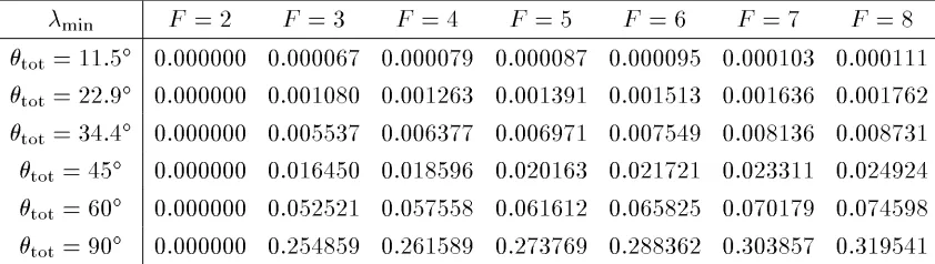
[image:24.612.95.516.121.240.2]

Table 2: Minimum eigenvalues for 1-D orthographic equi-angular motion with no constraint

5.3 More than two frames, without motion constraint

If we take the same data set as above, but remove the additional knowledge of equi-angular steps,

we end up solving for each motion (angle) estimate separately. The equations for

A

p

i,

A

p

i

m

j, and

A

m

j are given in (22–23), with

D = 0. Let us guess that the bas-relief ambiguity eigenvector has

the form

e

0= h

x0 ;z0 ;z N

;J J i

T

: (39)

The requirements for this to be an eigenvector are similar to those we derived before,

C;E = (40)

S;E = (41)

c

2

j

(jZ;W)+c j

s j

(2jW ;X ;Z)+s

2

j

(jX ;W) = j: (42)

In this case, we do not have a closed form solution, since we have2J+3equations in 3 unknowns.

However, if we assume a small angle approximation andW = 0(i.e., that the 3-D point cloud is

rotationally symmetric with respect to the middle frame), then the2J+1equations of the form (42)

are equivalent and we get the same eigenvectors as with the known equiangular motion constraint.

This behavior can be verified numerically (Table 2), where the results are quite similar to those

shown in Table 1. To obtain these results, we computed the

A

matrix explicitly using a set of 9 points sampled on the unit square, i.e., f(xz)xz 2 f;101gg, and then computed the

eigen-values. Note, however, that for an example whereW 6= 0, i.e., by adding one additional point at

(22)to the previous example, we get an eigenvector which is not of the form hypothesized in (39).

It is, however, an affine transform of the(x i

z i

(25)

6 Orthography: full 3-D reconstruction 17

S all

[image:25.612.136.476.120.240.2]

F =2 F =3 F =4 F =5 F =6 F =7 F =8 tot=11:5 1 123:61 113:80 108:18 103:50 99:34 95:60 tot=22:9 1 31:81 29:46 28:02 26:80 25:71 24:73 tot=34:4 1 14:88 13:88 13:21 12:62 12:09 11:62 tot=45 1 9:32 8:74 8:30 7:92 7:58 7:27 tot=60 1 6:01 5:65 5:35 5:08 4:85 4:64 tot=90 1 3:94 3:62 3:37 3:16 2:99 2:84

Table 3: S

allestimates for 1-D orthographic equi-angular motion with no constraint,

X =Z =100, =1.

We can also estimate the expected reconstruction errorS

allby summing the inverse

eigenval-ues. Using the same parameters as for Table 2, but withX = Z = 100 to make structure errors

dominate, we obtain the results in Table 3. This table shows how the bas-relief ambiguity dominates

the reconstruction error. At small viewing angles, doubling the angle results in a fourfold reduction

in the sum of squared errorS

all. Adding more frames is much less effective than increasing the

effective baseline of the system.

6 Orthography: full 3-D reconstruction

The situation with a regular orthographic camera (2-D retina, 3-D world) is quite similar to the

scanline camera. In this case, we use unit quaternions to represent the rotation matrices,

u ij

= r00 j

x i

+r01 j

y i

+r02 j

z

i (43)

v ij

= r10 j

x i

+r11 j

y i

+r12 j

z i

(44)

where the entries in the rotation matrixr

k lare given in (3).

To obtain a qualitative feel for the bas-relief ambiguity, let us examine the known equiangular

motion case with a small amount of rotation around a fixed axis (say in they-z plane),

q

j

1(0jq1jq2)] (45)

(26)

18 6 Orthography: full 3-D reconstruction

axis. As before, we ignore camera translations under orthography, since these can be recovered

from the motion of the point centroid.

The Jacobian matrix is now

H

T ij = 2 4 @u ij @x i @u ij @y i @u ij @z i @u ij @q 1 @u ij @q 2 @v ij @xi @v ij @yi @v ij @zi @v ij @q1 @v ij @q2 3 5 (46) 2 4

1 2jq2 ;2jq1 ;4j2q1x i

;2jz i

;4j2q2x i

+2jy i ;2jq2 1 2j2q1q2 2j2q2z

i

;2jx i

;4j2q2y i

+2j2q1z i

3 5

: (47)

The entries in the information matrix are

A

p

i 2 6 6 6 4

J0 0 0

0 J0 ;2J2q1q2 0 ;2J2q1q2 4J2q21

3 7 7 7 5 (48)

A

p

i

m

j 2 6 6 6 4

;4J2q1x i

;2J2q2x i ;2J2q2z

i

2J2q1z i 4J2q1z

i

;4J2q1y i 3 7 7 7 5 (49)

A

m

j = 2 4 4J2 P i z2 i ;4J2 P i y i z i ;4J2 P i y i z i 4J2 P i (x2 i +y2

i )

3 5

=4J2 2 4 Z W 0 W 0

X +Y 3 5

(50)

withY = P i y2 i, W 0 = P i y i z

i, and other terms as defined before.

These equations are similar to those for the orthographic scanline camera (22–23), withC J0,

S J2q21, E J2q1, and C 0

J2. In the absence of positional uncertainty, the accuracies of

theq1 andq2 estimates (

A

;1

m

j

) are inversely proportional toZ andX +Y, respectively, as is to be

expected. Similarly, with known motion, the triangulation error (

A

;1

p

i

) are inversely proportional

to the number of framesJ0 forxandy, and proportional to the squared rotation angleJ2q21 forz.

Notice that a non-zero tilt of the rotation axis (q2 6= 0) confounds some of theyandz positional

uncertainties.

Instead of trying to find an analytical solution to the eigenvalue problem, we present a brief

ex-ample showing the dependence ofmin onq1 andq2 (Table 4). For this example, we used a 15-point

data set consisting of the 8 corners of a unit cube, the 6 cube faces, and the origin. The eigenvalues

for the no-tilt case (q2 =0) are almost identical to the results of 1-D analysis (Table 2). The

eigen-values for the tilted case (q2=q1 = tan30 ) are similar in shape but show the effect of the overall

decrease inq1 values. By examining the eigenvectors (not shown here), we observe that for both

(27)

7 Perspective: single scanline 19

min F =2 F =3 F =4 F =5 F =6 F =7 F =8

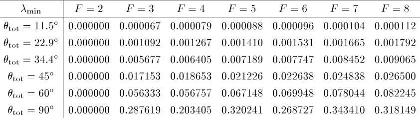
[image:27.612.96.517.121.240.2]

Table 4: Minimum eigenvalues for 2-D orthographic equi-angular motion with no constraint,

rota-tion aroundyaxis (q1=sin

j

2 ,q2 =0).

min F =2 F =3 F =4 F =5 F =6 F =7 F =8

Table 5: Minimum eigenvalues for 2-D orthographic equi-angular motion with no constraint,

rota-tion aroundyaxis tilted30 (q1 =cos30 sin

j

2 ,q2=sin30 sin

j

2 ).

7 Perspective: single scanline

Before analyzing the perspective camera in 3-D, let us briefly look at a perspective scanline (1-D)

camera. We can use this model to develop some intuitions, but unfortunately we cannot use it to

predict the performance of the full two-frame algorithm, since even under perspective, the scanline

camera has a bas-relief ambiguity. This can be shown by a simple parameter counting argument:

there are2N unknowns for the 2-D coordinatesf(x i

z i

)gand 1 (or more) unknowns for the motion,

but only2N measurements. In other words, we can place the cameras arbitrarily, and the

intersec-tions of the optical rays will determine the location of the 2-D points. This argument obviously does

[image:27.612.91.518.317.437.2]

(28)

20 7 Perspective: single scanline

min F =2 F =3 F =4 F =5 F =6 F =7 F =8

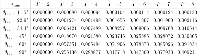
[image:28.612.94.517.121.240.2]

Table 6: Minimum eigenvalues for 1-D perspective projection, equi-angular rotation,=0:2.

conditioned.

The projection equation for a scanline camera, using the new projection model introduced in

(5), is u ij = c j x i ;s j z i +t xj 1+(s

j x i +c j z i +t z j ) = N ij D ij : (51)

The Jacobian matrix is

H

T ij = h @u ij @x i @u ij @z i @u ij @ j @u ij @t xj @u ij @t z j i (52) = 1 D ij h c j ;s j ~ u ij ;(s j +c j ~ u ij ) ;(s j x i +c j z i +(c j x i ;s j z i )~u ij

) 1 ;~u ij

i

whereu~

ij is the predicted value of u

ij computed by (51). In addition to the usual coordinate frame

ambiguity, we have a scale ambiguity, i.e., the(x i

z i

)andt

xj can be multiplied by a factor

a, andt z j

can be set toat z j

+(a;1)=, without affecting the solution. As mentioned above, a full bas-relief

ambiguity also exists for 2 frames.

Rather than continuing our analysis with the construction of the Hessian matrix

A

, let us just look briefly at the form of

H

ij. In addition to the terms already present under orthography (20), we

have the extra terms involving, as well as the partial with respect tot

z j. These additional terms

are what will, in full 3-D, enable the two-frame problem to be solved by removing the bas-relief

ambiguity.

To see the effects of using a perspective camera instead of an orthographic camera, we show

in Table 6 the minimum eigenvalue as a function of total viewing angle and number of frames.

Compared to Table 2, we see that there is a small, but not dramatic, improvement in the size of

(29)

8 Perspective in 3-D 21

min F =2 F =3 F =4 F =5 F =6 F =7 F =8

[image:29.612.94.516.121.240.2]

Table 7: Minimum eigenvalues for 3-D perspective projection, equi-angular rotation aroundyaxis,

=0:1.

8 Perspective in 3-D

Let us finally analyze the most interesting case, that of a perspective camera operating in a 3-D

environment. Here, we know that the two-frame problem has a solution, although our results on

the simpler camera models suggest that the reconstructions may be particularly sensitive to noise.

The forward imaging equations are given in (1–3) and (5). We will not bother deriving the

Ja-cobian and Hessian matrices here, as they are complex and not particularly informative. Instead,

we present some numerical results onmin andRMS

pos and discuss their significance. (Note that RMS

pos = S

pos =

p

n, wheren is the number of points.) These results were obtained using the

MathematicaR package [Wol91], by analytically differentiating the forward projection equations,

and then substituting in the known structure and motion parameters. Numerical eigenvalue analysis

was then used to obtain our results. For these examples, we used the 15 points sampled on the unit

cube described in Section 6.

We present results for two special cases: pure object-centered rotation (which in camera-centered

coordinates is actually both rotation and translation), and pure forward translation. Ignoring the

ef-fects of motion across the retina, these two cases capture the basic motion cues available to structure

from motion.

8.1 Pure object-centered rotations

To compute the minimum eigenvalue results, we used the same approach as for the orthographic 3-D

(30)

22 8 Perspective in 3-D

min =0:025 =0:05 =0:1 =0:2 =0:3 =0:4 =0:5

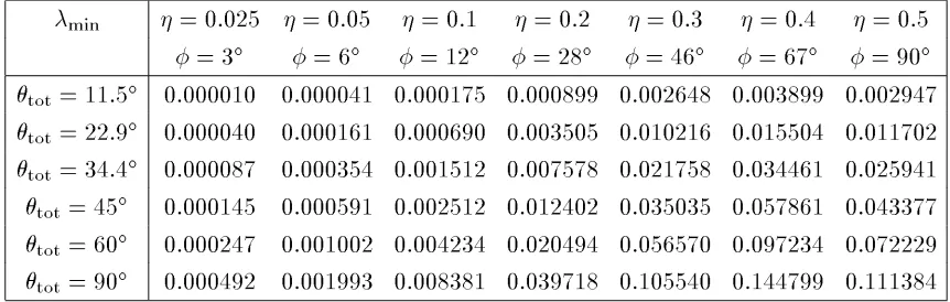
[image:30.612.90.521.121.258.2]

=3 =6 =12 =28 =46 =67 =90 tot=11:5 0:000010 0:000041 0:000175 0:000899 0:002648 0:003899 0:002947 tot=22:9 0:000040 0:000161 0:000690 0:003505 0:010216 0:015504 0:011702 tot=34:4 0:000087 0:000354 0:001512 0:007578 0:021758 0:034461 0:025941 tot=45 0:000145 0:000591 0:002512 0:012402 0:035035 0:057861 0:043377 tot=60 0:000247 0:001002 0:004234 0:020494 0:056570 0:097234 0:072229 tot=90 0:000492 0:001993 0:008381 0:039718 0:105540 0:144799 0:111384

two frames (F =2), varying. is the camera’s field of view.

case (Table 4), we see some striking differences. First, the two-frame problem is now soluble (up

to a scale ambiguity, of course). Second, for small viewing angles, there is marked improvement

even for multiple frames. Third, the results for large viewing angles with small’s are significantly

inferior to the orthographic results. This appears to be caused by ambiguities in camera motion

along the optical axis (t

z), which are neglected in the orthographic case.

This table only shows us the results for a particular value of. The dependence ofmin onis

presented in Tables 8 and 9 for the two and three frame problems. In these tables, the fields of view

equivalent to eachwere computed from the horizontal spread of the data points on the unit cube

and the distance of the cube from the camera

;1 using the formula

= 2tan ;1

1;

. As can be

seen for the two-frame case, doubling the amount of perspective distortion results in a fourfold

increase inmin (and hence a halving of the RMS error). For the three-frame case, the results are

less sensitive to.

What does a typical minimum eigenvector look like? Figure 5 shows the eigenvector

corre-sponding to the three-frame problem with=0:1and tot

=11:5 . As we can see, the majority of

the ambiguity is indeed a depth scaling. Notice, however, that the eigenvector is not a pure affine

transform of the 3-D coordinates, since the tips of the vectors in a given row do not form a straight

line (this has also been verified numerically). Our conjecture is that the minimum eigenvector may

be a projective transformation of the 3-D points, i.e., that the main ambiguity is projective, but we

have not yet found a proof for this conjecture.

How do the 3-D (position) errorsRMS

(31)

8.1 Pure object-centered rotations 23

min =0:025 =0:05 =0:1 =0:2 =0:3 =0:4 =0:5

[image:31.612.96.518.120.258.2]

=3 =6 =12 =28 =46 =67 =90 tot=11:5 0:000043 0:000075 0:000214 0:000956 0:002736 0:003908 0:002958 tot=22:9 0:000502 0:000688 0:001289 0:004384 0:011565 0:015655 0:011874 tot=34:4 0:001399 0:002606 0:004372 0:011820 0:028129 0:035277 0:026838 tot=45 0:001825 0:005074 0:009905 0:023998 0:052204 0:060488 0:046154 tot=60 0:002009 0:007177 0:020246 0:051574 0:103096 0:107273 0:082110 tot=90 0:002098 0:008302 0:032074 0:121672 0:205362 0:215310 0:181425

three frames (F =3), varying. is the camera’s field of view.

RMS pos

F =2 F =3 F =4 F =5 F =6 F =7 F =8 tot=11:5 20:78 19:08 18:04 17:02 16:12 15:32 14:62 tot=22:9 10:51 8:09 7:61 7:19 6:83 6:51 6:23 tot=34:4 7:13 4:64 4:38 4:13 3:94 3:75 3:60 tot=45 5:57 3:24 3:06 2:89 2:76 2:63 2:53 tot=60 4:35 2:32 2:19 2:07 1:98 1:89 1:82 tot=90 3:25 1:70 1:59 1:49 1:43 1:37 1:32

Table 10: RMS

pos for 3-D perspective projection, equi-angular rotation around

yaxis, =0:1.

By computing the full covariance matrix (inverting

A

) and taking the trace of the positional co-variance matrix

C

p

(as described in Section 3.2), we obtain the results shown in Table 10. These numbers indicate the relative errors in reconstruction for a unit retina and unit noise. For example,

if the retina is actually 200 pixels wide (s=100in (5)) and the positional error in the tracked points

is = 0:1, then the 3-D reconstruction errors would be 1000 times smaller than the values given

in Table 10. We see that this error decreases linearly with total viewing angle (for small viewing

angles), and varies only slightly with the total number of frames. This is similar to the results

ob-tained when computingmin in Table 4 (remember thatRMS error should be proportional to the

[image:31.612.140.473.343.463.2]

(32)

24 8 Perspective in 3-D

[image:32.612.120.506.70.292.2]

(a) (b)

Figure 5: Minimum eigenvector for a three-frame perspective reconstruction problem: (a)

top-down view (x-z), (b) frontal view (x-y). While the main ambiguity is a z scaling, the vector is

not exactly an affine transform of the 3-D points on the unit cube.

8.2 Looming

The motion of a camera forward in a 3-D world creates a different kind of parallax, which can also

be exploited to compute structure from motion. To compute the ambiguities in this kind of motion,

we used the same approach as before, except with no rotation and pure forward motion (t z

6=0).

Using our usual 15-point data set results in some unexpected behavior: four of the eigenvalues

are zero. This is because thezcoordinates of the three points on the optical axis cannot be

recov-ered as they lie on the focus of expansion. This is a severe limitation of recovering structure from

looming: points near the focus of expansion are recovered with extremely poor accuracy. For the

experiments in this section, we use a 12-point data set instead, i.e., the 15-point set with the three

points(xy)=(00)removed.

Table 11 showsmin as a function of the number of framesF and the total extent of forward

motiont

z (the object being viewed is a unit cube with coordinates

;11]3). These results are for

a camera with = 0:3, i.e., a camera placed about 3.3 units away from the cube origin. As we

can see, the two-frame results are almost as good at the three frame results with the same extent of

motion. The value ofmin appears to depend quadratically on the total extent of motion. Overall,

however, these results are much worse than those available with object-centered rotation.

(33)

9 Experimental results 25

min F =2 F =3 F =4 F =5 F =6

t z

=0:1 0:000007 0:000007 0:000007 0:000008 0:000009 t

z

=0:2 0:000027 0:000027 0:000030 0:000033 0:000037 t

z

=0:3 0:000060 0:000060 0:000067 0:000075 0:000084 t

z

=0:4 0:000107 0:000107 0:000119 0:000134 0:000150 t

z

[image:33.612.153.458.121.224.2]

=0:5 0:000168 0:000168 0:000187 0:000210 0:000235

Table 11: Minimum eigenvalues for 3-D perspective projection, pure forward translation,=0:3.

min =0:1 =0:2 =0:3 =0:4 =0:5

=12 =28 =46 =67 =90 t

z

=0:1 0:000000 0:000002 0:000007 0:000013 0:000020 t

z

=0:2 0:000001 0:000009 0:000027 0:000051 0:000078 t

z

=0:3 0:000002 0:000020 0:000060 0:000115 0:000176 t

z

=0:4 0:000004 0:000036 0:000107 0:000205 0:000314 t

z

=0:5 0:000006 0:000057 0:000168 0:000320 0:000490

Table 12: Minimum eigenvalues for 3-D perspective projection, pure forward translation,F =2,

varying.

appears thatmin depends cubically on , at least for small t

zs. To obtain reasonable estimates,

therefore, it is necessary to both use a wide field of view and a large amount of motion relative to

the scene depth.

Figure 6. shows the structural part of the minimum eigenvectors in particular for=0:3,J =1

(F = 3), andt z

=0:2. eigenvector whose 3-D structure is shown in Figure 6. By inspection of

the complete eigenvector (not shown here), we can see that the ambiguity is between the amount

ofxandyyaw andxandytranslation, i.e., it is a classic bas-relief ambiguity.

9 Experimental results

To verify if the positional errors predicted by our analysis coincide with the errors observed in

[image:33.612.153.457.275.397.2]

(34)

26 9 Experimental results

[image:34.612.83.541.62.307.2]

(a) (b)

Figure 6: Minimum eigenvector for a three-frame perspective reconstruction problem with pure

z translation: (a) top-down view (x-z), (b) frontal view (x-y). The main ambiguity is a rocking

confusion between sideways camera translation and rotation, which affects the points furthest back.

The 24 points were four points at(0:46850:4685)on the six faces of a unit;1+1]3 cube. The

points were projected onto a 200 pixel wide retina (s=100in (5)) and 2-D noise with =0:1was

added to each projected point.5 The algorithm was then initialized with the correct 3-D structure

and run to completion.

The 3-D positional errors are shown in Tables 13 and 14. Three kinds of error are shown: the

Euclidean error, after registering the recovered and true 3-D data sets under the best possible

sim-ilarity transform (rigid+scaling); the affine error (computing the best affine transform); and the

projective error (computing the best44homography). These errors were scaled by a factor of

1000 to make them “dimensionless” (i.e., unit retina, unit image noise). The RMS error predicted

by our uncertainty analysis (the trace of the positional covariance matrix) is also shown.

From these results, we can see that the uncertainty analysis predicts the general variation of

re-construction error with viewing angle, perspective distortion, and number of frames. Unfortunately,

there remains a small but fairly consistent discrepancy between our predicted figures and the

mea-sured errors, which we have not been able to track down. We also see that the affine error is about

2 to 3 times lower than the Euclidean error (actually, this factor increases with decreasing viewing

5

The results scale linearly withup to about = 1, after which they increase sub-linearly (i.e., they less than

(35)

10 Discussion 27

RMS pos

=0:1 =0:2

[image:35.612.86.528.120.241.2]

F =2 predicted Euclidean affine projective predicted Euclidean affine projective tot=8 35:02 58:98 20:41 19:02 19:68 34:43 21:68 20:48 tot=16 18:21 35:70 10:27 9:39 9:93 16:63 10:39 9:75 tot=32 9:28 15:70 5:10 4:78 5:13 9:15 5:34 4:98 tot=60 5:24 8:47 2:89 2:72 3:02 4:69 3:01 2:82 tot=90 3:85 5:36 2:03 1:93 2:37 3:32 2:15 2:04

Table 13: RMS errors (predicted and observed) for 3-D perspective projection, equi-angular

rota-tion aroundyaxis, two frames, 24 point data set.

RMS pos

=0:1 =0:2

F =3 predicted Euclidean affine projective predicted Euclidean affine projective tot=6 41:94 61:17 20:21 18:76 25:79 40:45 22:21 20:26 tot=12 19:83 26:90 10:31 9:69 12:55 18:12 10:39 9:71 tot=24 7:42 11:34 4:99 4:76 5:75 8:08 5:23 4:91 tot=48 2:76 3:70 2:50 2:43 2:59 3:63 2:72 2:61 tot=90 1:59 1:96 1:54 1:50 1:57 1:90 1:59 1:53

Table 14: RMS errors (predicted and observed) for 3-D perspective projection, equi-angular

rota-tion aroundyaxis, three frames, 24 point data set.

angle, as predicted by our analysis). The projective error is not significantly lower than the affine

error, which further supports our hypothesis that most of the error is in the bas-relief ambiguity.6

10 Discussion

The results presented in this technical report suggest that in many situations where structure from

motion might be applied, the solutions are extremely sensitive to noise. In fact, despite dozens

of algorithms having been developed, very few results of convincing quality are available. Those

6

[image:35.612.86.527.311.432.2]

(36)

28 10 Discussion

cases where metrically accurate results have been demonstrated almost always use a large amount

of rotation [TK92b].

This raises the obvious question: are any of the many structure from motion algorithms

de-veloped in the computer vision community of practical significance? Or, when we wish to perform

metrically accurate reconstructions from images, should be adopt the photogrammetrists’ approach

of using control points at known locations? This essentially reduces structure from motion to

cam-era pose estimation (and possibly calibration) followed by stereo reconstruction.

The situation is perhaps not that bad. For large object rotations, we can indeed recover accurate

reconstructions. Furthermore, for scene reconstruction, using cameras with large fields of view,

several camera mounted in different directions, or even panoramic images, should remove most of

the ambiguities. In any case, it would appear prudent to carefully analyze the expected ambiguities

and uncertainties in any structure from motion problem (or any other image-based estimation task)

before actually putting a method into practice.

The general approach developed in this technical report, i.e., eigenvalue analysis of the Hessian

(information) matrix appears to explain most of the known ambiguities in structure from motion.

However, there are certain ambiguities (e.g., depth reversals under orthography, or multiplicities of

solutions with few points and frames) which will not be detected by this analysis because they

cor-respond to multiple local minima of the cost function in the parameter space. Furthermore, analysis

of the information matrix can only predict the sensitivity of the results to small amounts of image

noise. Further study using empirical methods is required to determine the limitations of our

ap-proach.

Using the minimum eigenvalue to predict the overall reconstruction error may fail when the

dominant ambiguities are in the motion parameters (e.g., what appears to be happening under

per-spective for large motions). Computing theRMS

pos error directly from the covariance matrix

A

;1

is more useful in these cases.

10.1 Future work

In future work, we plan to compare results available with object-centered and camera-centered

rep-resentations (Equations 4–5). Our guess is that the former will produce estimates of better quality.

Similarly, we would like to analyze the effects of mis-estimating internal calibration parameters

(37)

11 Conclusions 29

process. The results presented here have assumed for now that feature points are visible in all

im-ages. Our approach generalizes naturally to missing data points. In particular, we would like to

study the effects feature tracks with relatively short lifetimes.

Finally, it appears that the portion of the uncertainty matrix which is correlated can be accounted

for by a small number of modes. This suggest that an efficient recursive structure from motion

algorithm could be developed which avoids the need for using full covariance matrices [THO93]

but which performs significantly better than algorithms which ignore such correlations.

11 Conclusions

This technical report has developed new techniques for analyzing the fundamental ambiguities and

uncertainties inherent in structure from motion. Our approach is based on examining the

eigenval-ues and eigenvectors of the Hessian matrix in order to quantify the nature of these ambiguities. The

eigenvalues can also be used to predict the overall accuracy of the reconstruction.

Under orthography, the bas-relief ambiguity dominates the reconstruction error, even with large

numbers of frames. This ambiguity disappears, however, for large object-centered rotations. For

perspective cameras, two-frame solutions are possible, but there must still be a large amount of

ob-ject rotation for best performance. Using three of more frames avoids some of the sensitivities

asso-ciated with two-frame reconstructions. Translations towards the object are an alternative source of

shape information, but these appear to be quite weak unless large fields of views and large motions

are involved.

When available, prior information about the structure or motion (e.g., absolute distances,

per-pendicularities) can be used to improve the accuracy of the reconstructions. Whether 3-D

recon-struction errors (for modeling) or motion estimation errors (for navigation) are most significant for

a given application determines the conditions which produce acceptable results. In any case,

care-ful error analysis is essential in ensuring that the results of structure from motion algorithms are

sufficiently reliable to be used in practice.

References

(38)

30 11 Conclusions

noisy flow field. IEEE Transactions on Pattern Analysis and Machine Intelligence,

11(5):477–490, May 1989.

[AHP93] A. Azarbayejani, B. Horowitz, and A. Pentland. Recursive estimation of structure and

motion using relative orientation constraints. In IEEE Computer Society Conference

on Computer Vision and Pattern Recognition (CVPR’93), pages 294–299, New York,

New York, June 1993.

[Aya91] N. Ayache. Artificial Vision for Mobile Robots: Stereo Vision and Multisensory

Per-ception. MIT Press, Cambridge, Massachusetts, 1991.

[CT92] Q. Chen and S. Tsuji. A hierarchical method that solves the shape and motion from

an image sequence problem. In IEEE/RSJ Int’l Conference on Intelligent Robots and

Systems, pages 2131–2138, July 1992.

[CWC90] N. Cui, J. Weng, and P. Cohen. Extended structure and motion analysis from

monocular image sequences. In Third International Conference on Computer Vision

(ICCV’90), pages 222–229, Osaka, Japan, December 1990. IEEE Computer Society

Press.

[DA90] C. H. Debrunner and N. Ahuja. A direct data approximation based motion estimation

algorithm. In 10th Int’l Conference on Pattern Recognition, pages 384–389, 1990.

[Fau92] O. D. Faugeras. What can be seen in three dimensions with an uncalibrated stereo

rig? In Second European Conference on Computer Vision (ECCV’92), pages 563–

578, Santa Margherita Liguere, Italy, May 1992. Springer-Verlag.

[HG93] R. Hartley and R. Gupta. Computing matched-epipolar projections. In IEEE

Com-puter Society Conference on ComCom-puter Vision and Pattern Recognition (CVPR’93),

pages 549–555, New York, New York, June 1993. IEEE Computer Society.

[HGC92] R. Hartley, R. Gupta, and T. Chang. Stereo from uncalibrated cameras. In IEEE

Com-puter Society Conference on ComCom-puter Vision and Pattern Recognition (CVPR’92),

pages 761–764, Champaign, Illinois, June 1992. IEEE Computer Society Press.

[Hor90] B. K. P. Horn. Relative orientation. International Journal of Computer Vision,

4(1):59–78, January 1990.

[KTJ89] R. V. R. Kumar, A. Tirumalai, and R. C. Jain. A non-linear optimization algorithm for