Pressure derivative analysis for horizontal wells in shale reservoirs under trilinear flow conditions

www.arpnjournals.com

PRESSURE DERIVATIVE ANALYSIS FOR HORIZONTAL WELLS IN

SHALE RESERVOIRS UNDER TRILINEAR FLOW CONDITIONS

Freddy Humberto Escobar, María Alejandra Cabrera and Astrid Juliana Ortiz

Universidad Surcolombiana/CENIGAA, Avenida Pastrana, Neiva, Huila, Colombia

E-Mail: fescobar@usco.edu.co

ABSTRACT

Unconventional shale reservoirs appear as a solution to the depletion of conventional reserves, however, their ultra low permeability, requires hydraulic fracturing that helps improving the fluid flow towards the well. The design and creation of these fractures is complex. Knowing their properties, and the reservoir´s, as well, is of great importance for field management. This study presents a practical methodology for well test interpretation in shale reservoirs using the analytical trilinear flow model, which describes a system consisting of a horizontal well with multiple fractures in extremely low permeability reservoirs. Analytical expressions were developed based upon unique features found on the pressure and pressure derivative curves for the determination of fracture conductivity (kFwF), half-fracture length (xF), matrix permeability (km) and internal reservoir permeability (kI). Finally, synthetic examples for both oil reservoirs and gas formations were developed to successfully verify the accuracy of the developed equations.

Keywords: unconventional resources, shale reservoirs, hydraulic fractures, trilinear flow model, TDS technique.

1. INTRODUCTION

In the continuous search to increase hydrocarbon production under the high global energy demand, the world has currently turned its attention to non-conventional deposits. There several types of unconventional resources; one of them refers to shales. What makes shales their unconventional character is their ultra-low permeability, that can oscillate between 10-6 _and 10-12 _{darcies, but generally is given in the order of} nanodarcies (10-9 _{darcies) and possess small pore} diameters that oscillate between 1 and 10 μm, explaining why they commonly are considered as impermeable. Exploitation of these types of reservoirs requires long horizontal wells and the implementation of a good hydraulic fracturing job, with the solid purpose of creating extensive networks of artificial fractures, to increase the well productivity index and to optimize the recovery of reserves.

Prats (1961) and Prats, Hazebroek and Strickler (1962) began studying the effect of vertical fractures on the behavior of the reservoirs. Ramey and Raghavan (1974) presented a solution for a vertical fracture of infinite conductivity in a vertical well. Based on the above, Cinco-Ley, Samaniego and Dominguez (1978) did the same for a finite-conductivity fracture. Cinco-Ley and Samaniego (1981) analyzed the transient pressure behavior of finite-conductivity fractured wells and found a new flow regime called bilinear. Camacho (1984), Bennett et al. (1985), Camacho, Raghavan and Reynolds (1987) who obtained transient pressure analytical solutions for a vertical well intercepted by a finite-conductivity vertical fracture in naturally fractured reservoirs. Cinco and Meng (1988) presented semi-analytical model for finite-conductivity fractured wells in naturally occurring formations with both transient matrix flow and pseudosteady state matrix flow. They mentioned a trilinear flow formed by a matrix linear flow superimposed to the bilinear flow in the formation-fracture system.

The trilinear flow model, Brown et al. (2009), divides the reservoir into three zones with average properties: internal reservoir, external reservoir and hydraulic fractures. Their solution of the diffusivity equations was obtained in the Laplace domain space separately for each zone and the calculated results in the Laplace domain were reversed again in the time domain using the Stehfest algorithm (1970). Al-Hussainy and Ramey (1966) and Al-Hussainy, Ramey and Crawford (1966) introduced the idea of gas pseudopressure in order to give an analytical solution to gas deposits. Because the internal reservoir is a naturally fractured medium, the dual porosity model of Kazemi (1969), De-Swaan (1976) and Serra, Reynolds and Raghavan (1983) form the basis of the trilinear flow model. In addition, the model assumes that the productive life of a fractured horizontal well depends on the volume of hydraulic fractures, Raghavan, Chen and Agarwal (1997).

The behavior of fluids within a reservoir composed of very tight matrix, hydraulic fractures and natural fractures (usually induced at the time of hydraulic fracturing), in a horizontal well, can be interpreted using an analytical model known as trilinear flow model, formulated and verified by Brown (2009) and Brown et al. (2009). As implied by its name, the trilinear flow model assumes three linear flows during the productive life of the well and its interpretation was based on a series of previous work on the behavior of fluids in porous media, as well as in vertical and horizontal wells in naturally and/or hydraulically fractured reservoirs.

developed equations were successfully tested with synthetic examples.

Figure-1. Schematic representation of the trilinear flow model with three continuous flow regions for a horizontal

multi-fractured well, Brown, M. (2009).

2. MATHEMATICAL MODEL

The trilinear flow model formulated by Brown (2009) and Brown et al. (2009) assumes linear flow in three different reservoir zones: internal deposit, external deposit and hydraulic fractures, as shown in Figure-1. The remaining model assumptions can be found in Brown et al. (2009).

The analytical dimensionless pressure solution for a horizontal multi-fractured well, Brown et al. (2009), is given by:

 

0

( )

tanh

D

D _{FD x}

FD F F

P P

sC 

 



  (1)

Other model-related parameters are provided in Appendix A. The dimensionless oil pressure and pressure derivative are given by:

,

( )

141.2

D

I

i wf

F sc

k h

P P P

q B

  (2)

,

* ' ( * ')

141.2 I

D D

F sc

k h

t P t P

q B

  (3)

For gas Wells,

 

 

 

, 1422

I

i wf

D

F Msc

k h

m P m P m P

q T 

 _  _ (4)





,

* ( ) ' * ( )'

1422.52 I

D D

F Msc k h

t m P t m P

q T

  (5)

m(P) is a gas pseudopressure function, Al-Hussainy et al. (1966); Al-Hussainy and Ramey (1966); given by:

'

( ) 2 '

b P

P

P

m P dP

z 



_

(6)

The dimensionless time is:

2

0.0002637 ( )

I D

t I F

k t t

c x

 

 (7)

Some dimensionless variables related to reservoir geometry and fractures are:

e D

F

x x

x

 (8)

e D

F

y y

x

 (9)

F D

F

w w

x

 (10)

3. WELL PRESSURE BEHAVIOR

As mentioned before, three cases can take place:

Case 1 considers three characteristic flow regimes (Figure-2). A bilinear flow regime is observed at early time. This occurs once the transient wave detects two simultaneous linear flow regimes in the fractures and inner reservoir, respectively. A second linear flow (first linear) appears in response the fluid flow from the natural fracture network to the hydraulic fractures. Finally, a (first) pseudosteady-state period is because the matrixes do not feed the natural fractures. Generally, the first linear flow can be seen when the  product is les or equal to 1, or simply when  and  take very low values which ensures the flow incapability from matrix to induced natural fractures. Because  is matrix permeability independent, this case normally takes place when the mentioned permeability value is ultra-low enough (<1x10-9_{) so the} pressure in the test changes linearly with time.

Case 2 involves the acting of five flow regimes (Figure-2): Bilinear, first linear and first pseudosteady-state period of case 1; then, second linear and second state. Followed by the first pseudosteady-state period, and after a considerable response time, the pressure changes linearly with time and the second linear flow can be observed; once the transient wave reaches the hydraulic fracture limits or the internal reservoir boundary, the second pseudosteady-state period is developed. There exists a certain relationship between - and the second linear flow regime. Frequently, when  has large values, the second linear flow becomes visible in the pressure derivative versus dimensionless time log-log plot; when  grows, the duration of the second linear flow also does so, and this, in turn, occurs late, as becomes small.

Line of symmetry No-Flow Line

No-Flow Boundary ye=dF/2

xF

xe

y x OUTER

RESERVOIR ΦO, CtO, KO Φm, Ctm, Km

INNER RESERVOIR NATURALLY FRACTURED ΦI, CtI, KI Φf, Ctf, Kf HYDRAULIC

FRACTURE ΦF, CtF, KF

www.arpnjournals.com

In Case 3 is possible to differentiate three flow regimes (Figure-2): at early times, a bilinear flow is observed, later a linear flow, the same that we have called the second linear flow in case 2, followed by a pseudosteady or second pseudosteady state. This case is given due to the simultaneous movement of matrix fluids to natural fracture and natural fracture to hydraulic fracture, under conditions of large  and  values.

1.E-02 1.E-01 1.E+00 1.E+01 1.E+02 1.E+03 1.E+04 1.E+05 1.E+06 1.E+07 1.E+08

1.E-04 1.E-03 1.E-02 1.E-01 1.E+001.E+011.E+021.E+031.E+04 1.E+051.E+061.E+071.E+08

t * P ' D D Case 2 Case 3 Case 1 Bilinear flow m = 0.25

1st linear m = 0.5

2nd linear m = 0.5 1st pseudosteady

m = 1

2nd pseudosteady m = 0.5

tD

Figure-2. Dimensionless pressure derivative behavior for a reservoir under trilinear flow conditions with case 1,

case 2 or case 3.

3.1. TDS TECHNIQUE FOR OIL SHALE

RESERVOIRS

Bilinear flow regime. The governing equation developed for this flow regime is:

0.5 0.25 1

( * ')

1.6289 BL

F I f f

D D BL D

F F

x k h

t P t

k w 

 

  

  (11)

Replacing the dimensionless quantities, Equations 3 and 7 into Equation 11 and solving for the fracture conductivity, kFwF:

0.5 1.5 2 , 122.0157 ( ) ( * ') BL

F F f f

I t I

F scB

BL

t

k w h

k c

q h t P

      _{ }      _    (12)

First linear flow regime:The governing equation for the first linear flow is:





1 ₁

0.5

1.1 1 * '

360 L

D D L D

t P  t (13)

Replacing dimensionless variables and solving for the internal reservoir permeability, kI:

 





2 , 1 1 4.0739 * ' F sc L I

t I F L

q B

t k

c x h t P

         

  (14)

First pseudosteady-state period: The governing equation for the first pseudosteady-state is:



D '



1 ₂ pss1

e

pss D

F D

x

t P t

y





 (15)

Again replacing the dimensionless parameter and solving for half-fracture length, xF:

  

, 1



1

1

17.0966 * '

F sc pss F

e t I pss

q Bt x

y h c t P 

 (16)

Second linear flow: Its governing equation is:





2

0.5 0.5 2 ( ) 1 * '

2.2783 ( ) L I

f I t

D D D

e m t m

L

h k c

t P t

y k c

 

 

 _{ }

  (17)

The matrix permeability, km, is solved for once the dimensionless quantities are replaced in the above expression:

 





2 , 2 2 1.0128 '

F sc f L

t m F L

m

e

q Bh t

k

c x y h t P

 

 

  _{ } 

 

  (18)

The Second pseudosteady-state period has the following governing Equation:



'



2 1.5511

_{ }

 

pss2

F f t I

pss

D D D

e m t m

c

t P t

y h c x h 





 (19)

Which allows finding an expression for determining the half-fracture length, xF, once the dimensionless variables are used:





,

2 2

1

17.3145 ( ) * '

f pss F sc F

e m t m p ss

y c t P

q Bh t x

h h



 (20)

3.2 TDS TECHNIQUE FOR GAS SHALE RESERVOIRS

The Bilinear flow regime governing equation is:



_{* ( )}



1 0.5 0.25

1.628 '

9 BL

F I f f

D D BL D

F F

x k h

t m P t

k w 

 

  

  (21)

 

 





0.5 2 , 1 2384.0667 * ' BL

F F f f

I t I

F Msc

BL

t

k w h

k c

q T

h t m P

                     (22)

The governing equation for the First linear flow regime is:





1

0.5

1 _1.1360

1 * ( ) '

L

D D L D

t m P  t (23)

After replacing the dimensionless variables leads to find the internal reservoir permeability, kI:

 





2 , 1 1 413.4878 ( ) ' F Msc L I

t I F L

q t

c x t

T h m k P       _{ }   

  (24)

First pseudosteady-state period: The governing equation for the firstpseudosteady-state is:



* ( ) '



1 ₂ pss1

F

D D pss D

e

x

t m P t

y 

 (25)

Replacing the dimensionless parameter and solving for half-fracture length, xF:

 

,



1

 



1

1

1.6971 '

F Msc ps F

s

e t I pss

q t

y h c t m P

T x

 



 (26)

The second linear flow has the following governing equation:





2

0.5 0.5 2 _2. ( ) 1 * ( ) '

2783 ( ) L

f I t

D D L D

e

I

m

m t

h k c

t m P t

y k c

 

 

 _{ }

  (27)

Replacing the dimensionless terms in the above expression leads to solve for the matrix permeability, km:

 





2 , 2 2 102.8034 ( ) ' F Msc L

t F e L

f m m Th q t k h

c x y t m P

 

 

  _{ } 

 

  (28)

The governing equation of the Second pseudosteady-state period is given by:



* ( ) '



2 1.5511

_{ }

 

pss2

F t I

D D pss D

m f

m

e t

c

t m P t

y h c x h 



 (29)

Replacing the dimensionless terms and, then, solving for the half-fracture length, xF, will result:

 

,



2

 



2

1

1.7187 '

F Msc f pss

e m t _pss

F

m

q h t

y h h c t

T x

m P  



 (30)

Intersection points

The equations resulting from the points of intersection of the different flows are the same for both gas and oil reservoirs.

Intersection of first pseudosteady-state and bilinear flow:





 

3 2 4 9 1

1.2719 10 f f t I

I F e

F F pss BLi

h c

k x y

k w t

                  

 (31)

Intersection of first pseudosteady state and linear flow:

 

0.5 1 1 1 34.5077

I pss L i e t I k t y c          

  (32)

Intersection of bilinear-first linear:

 

0.5

2

1

29.9503 t I I

F F F f f

Bl L i

c k

k w x h

t        _{ }

  (33)

Intersection of second pseudosteady-state and bilinear flow:

 

 

2 2 9 3 4

1.34 10 e m t

I

t

f

F F pss BL

F m

i I

f

y h c k w x h c k t                          (34)

Intersection of second pseudo steady state and second linear flow:

 

2

2 2

303.6558 m t

pss L i

m m

k h c

t  



 (35)

Intersection of bilinear-second linear:

2 0.5

2 2 _{( )}

120.4702

( )

f t m

F F

f t I I BLL

e F m

i

y x

k

k c

k w

h c t

  

 _

 

 _{ }

  (36)

Intersection of second pseudosteady state and first linear:

 

 

0.5 2 1

34.9485

1 f I t I pss L i e

m t m

c t y

h c

h k 

 



 

 _{ }

 

www.arpnjournals.com

Intersection of second linear with first pseudosteady state

 

2

2 1

296.0935 ( )

m f t I

t m L pss i

k h c

c t

 _

 _  

 _{ } (38)

4. SYNTHETIC EXAMPLES

The worked examples used data from Bowen et al. (2009).

4.1. Example 1

A pressure test was simulated for an oil reservoir drained by a horizontally fractured hydraulic well (Figure-3) and data presented in Table-1. Estimate: the half-fracture length, hydraulic half-fracture conductivity and permeability of the natural fractures.

Solution: The following computations are performed using Equations A-9, A-11 and A-12:

λ = 2.0758Χ10-10_{, ω =0.00333333, Ƞ}

O = 6.2786Χ10-12 md-psi/cp, ȠI = 10.4642857 md-psi/cp and ȠF =

5806026.32 md-psi/cp.

Case 1 is confirmed from Figure-3 from which the following characteristic points were read:

tBL = 0.0119 hr ΔPBL = 4.82Χ10-3 psi (t*ΔP’)BL = 1.21Χ10-3 psi tpss1 = 4760 hr

ΔP pss1 = 0.887 psi (t*ΔP’)pss1 = 0.812 psi tL1 = 13.1 hr ΔPL1 = 0.033psi

(t*ΔP’)L1 = 0.012 psi tpss1-L1i = 360.7915 hr tpss1-L1i =60.8027 hr tBL-L1i = 1.624014 hr

Find the fracture conductivity, kFwF, with Equation 12, natural fractured network permeability, kI, form Equation 14 and half-fracture length, xF, with Equation 16, so that:

3

1

1 34.83*1.35*4.76*10 17.0966 1 08.5*380*0.7*0.006*8.12*10

F

x  _

1.E-03 1.E-02 1.E-01 1.E+00 1.E+01

1.E-02 1.E-01 1.E+00 1.E+01 1.E+02 1.E+03 1.E+04 1.E+05

t , hr



P

and

t*



P

', psi

  _{1 21 10 psi}3

BL

t* P'_{ }. _ 

0.0119 hr

BL

t 

 PL10 033 psi.

1 13.1hr

L

t 

t* P'L10 012 psi.

1 (t* P')pss0 812 psi.

 Ppss10 0104 psi.

3 1 4.76 10 hr

pss

t  

Figure-3. Pressure and pressure derivative vs. Time log-log plot for example 1 (oil reservoir).

Table-1. Input data for examples 1 and 2 Brown, M. (2009).

Parameter Example 1 Example 2

h, ft 380 250

rw, ft 0.3 0.3

ye, ft 108.5 250

xe, ft 7500 500

μ, cp 0.3 0.0184

km, md 5Χ10-16 1Χ10-6

m, fraction 0.07 0.05 ctm, psi-1 0.000001 0.00001

hm, ft 1 1.25

kf, md 50 2000

f, fraction 0.7 0.45 ctf, psi-1 0.006 0.00001

hf, ft 0.005 0.001

F, fraction 0.38 0.38

kF, md 25100 1*105

ctF, psi-1 0.00001 0.00001

wF, ft 0.01 0.01

xF, ft 93 250

qF, STB/D or Mscf/D 34.83 100

Bo 1.35 1.35

ρf, f/ft 1 0.8

T, °R 600 610.67

93.1035 ft

F

x 

2 1

2

1.31*10 *0.3 34.83*1.35 4.0739

0.7 *0.006 93*380*1.20*10

I

k  _{ } _

 

46.8633 md

I

k 

0.5 2 1.5

2

3

1.19*10 122.0157*0.005*1*0.3

50*0.7*0.006

34.83*1.35

249.5560 md-ft 380*1.21*10

F F

k w





 

 _{ }

 

 _{ }

 

 

Find natural fracture permeability, kI, with Equation 31, reservoir length, ye, using Equation 32 and fracture conductivity, kFwF, with Equation 33.

0.5

1 360.7915

109.6601 ft 34.5077 0.3 *0.7 *0.00

0

6 5 *

e

y  _ _ 

2

9 4

3

0.005*1 1.2719 *10 *93*108.5

251 0.3* 0.7 * 0.006

*

46.5643 md 60.8027

I

k  _ _

 



 

 

 

0.5 2 0.3*0.7*0.006*50

29.9503*93 *0.005*1*

1.6240

F F

k w  _ _

 

255.1012 md-ft

F F

[image:6.612.72.532.56.462.2]

k w 

Table-2. Comparison of results for example 1.

Equation Parameter Input This work Error, %

12 kFwF, md-ft 251 249.5560 0.58 14 kI, ft 50 46.8633 6.27

16 xF,ft 93 93.1035 0.11

31 kI, md 50 46.5643 6.87 32 ye, ft 108.5 109.6601 1.07 33 kFwF, md-ft 251 255.1012 1.63

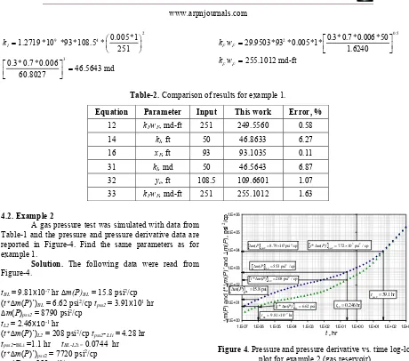
4.2. Example 2

A gas pressure test was simulated with data from Table-1 and the pressure and pressure derivative data are reported in Figure-4. Find the same parameters as for example 1.

Solution. The following data were read from Figure-4.

tBL = 9.81Χ10-7 hr Δm(P)BL= 15.8 psi2/cp (t*Δm(P)’)BL = 6.62 psi2/cp tpss2 = 3.91Χ101 hr

Δm(P)pss2 = 8790 psi2/cp tL2 = 2.46Χ10-1 hr

(t*Δm(P)’)L2 = 208 psi2/cp tpss2-L1i = 4.28 hr tpss2-BLi =1.1 hr tBL-L2i = 0.0744 hr

(t*Δm(P)’)pss2 = 7720 psi2/cp

Δm(P)l2 = 553psi2/cp

1.E+00 1.E+01 1.E+02 1.E+03 1.E+04 1.E+05 1.E+06

1.E-07 1.E-06 1.E-05 1.E-04 1.E-03 1.E-02 1.E-01 1.E+00 1.E+01 1.E+02 1.E+03

t , hr

t* m P( )'BL6 62 psi.

7 9.81 10 hr

BL t _{ } 

m P( )_BL15 8 psi.

2 0.246 hr

L t 

  2 2 ( )L 553 psi cp

m P /

 

  2 2 ( )'L 208 psi cp

t* m P  /

2 39.1hr

pss

t 

  3 2 2

( )pss 7 72 10 psi cp

t* m P ' .  /

  3 2 2

( )pss 8 79 10 psi /cp

m P .

  



m

(

P

)

a n dt*

m

(

P

)

'

a n dm

(

P

), p

si

/cp



Figure 4. Pressure and pressure derivative vs. time log-log plot for example 2 (gas reservoir).

[image:6.612.275.539.151.440.2]

Using Equations 22 and 36, 28 and 35, 30 and 34, fracture conductivity, kFwF, matrix permeability, km, half-fracture length, xF and natural fractured network permeability, kI, were estimated and reported in Table-3.

Table-3. Comparison of results for example 2.

Equation Parameter Input This work Error, %

22 kFwF, md-ft 1000 1002.885 0.29 28 km, md 1x10-6 9.86x10-7 1.40

30 xF,ft 250 250.381 0.15

34 kI, ft 2000 2076.767 3.69 35 km, md 1x10-6 1.02x10-6 2.00 36 kFwF, md-ft 1000 986.511 1.35

5. CONCLUSIONS

a) New equations are presented to characterize systems consisting of a horizontal well with multiple fractures in ultra-low permeability reservoirs using characteristic points found on the pressure derivative so natural fracture permeability, matrix permeability,

half-fracture length and hydraulic fracture conductivity can be estimate and verified.

[image:6.612.167.442.546.656.2]

www.arpnjournals.com

regimes are: bilinear, first linear, first pseudosteady-state, second linear and second pseudosteady-state. Finally, for case 3, the observed flow regimes are: bilinear, followed by a linear and pseudosteadystate -same called as second linear and second pseudosteady-state in case 2, which can be identified from such properties as matrix permeability and the resulting values of the interporosity flow parameter and the dimensionless storativity ratio.

Nomenclature

B Formation volume factor, rb/STB, ft3_/SCF CFD Hydraulic fracture conductivity, dimensionless CRD Reservoir conductivity, dimensionless ct Total compressibility, 1/psi

dF Distance between two adjacent fractures, ft h Reservoir thickness, ft

hf Thickness of natural fractures, ft hft Total thickness of natural fractures, ft hm Thickness of matrix slabs, ft

k Permeability, md

kf Natural fracture intrinsic permeability, md kF Hydraulic fracture permeability, md kI Permeability of the inner reservoir, md kO Permeability of the outer reservoir, md km Matrix intrinsic permeability, md m(P) Pseudopressure, psi2_/cp

nF Number of hydraulic fractures nf Number of natural fractures P Pressure, psia

PD Dimensionless pressure Pi Initial reservoir pressure, psi q Flow rate, STB/d

qF,sc Flow rate for a hydraulic fracture, oil STB/d, gas Mscf/d

S Laplace parameter t Time, hr

T Reservoir Temperature, °R tD Dimensionless time

tD*PD’ Dimensionless pressure derivative tD*m(P)D’Dimensionless pseudopressure derivative t*Δm(P) Pseudopressure derivative, d/Mscf wF Hydraulic fracture width, ft xe Reservoir size, x-direction, ft xF Hydraulic half-fracture length, ft ye Reservoir size, y-direction, ft z Real gas- compressibility factor

Greek

α Parameter defined in trilinear flow model β Parameter defined in trilinear flow model Δ Difference operator

ф Porosity, fraction ƞ Diffusivity, ft2/hr

λ Transmissivity ratio, transient dual porosity model

μ Viscosity, cp π Pi Constant

ρf density of natural fractures, fractures/ft ω Storativity ratio, transient dual porosity model

Subscripts

BL Bilinear flow D Dimensionless e External boundary f Natural fracture F Hydraulic fracture i Initial

I Inner Reservoir m Matrix

L1 First linear flow L2 Second linear flow O Outer Reservoir pss1 First pseudosteady state pss2 Second pseudosteady state R Reservoir

Sc Standard conditions t Total

wf Flowing wellbore ξ type of medium: L,F,O

REFERENCES

[1] Al-Hussainy R. & Ramey H. J. 1966, May 1. Application of Real Gas Flow Theory to Well Testing and Deliverability Forecasting. Society of Petroleum Engineers. doi: 10.2118/1243-B-PA.

[2] Al-Hussainy R., Ramey H. J. & Crawford P. B. 1966, May 1. The Flow of Real Gases through Porous Media. Society of Petroleum Engineers. doi: 10.2118/1243-A-PA.

[3] Bennett C. O., Camacho-V., R. G., Reynolds A. C. & Raghavan R. 1985, October 1. Approximate Solutions for Fractured Wells Producing Layered Reservoirs. Society of Petroleum Engineers. doi: 10.2118/11599-PA.

[4] Brown M. 2009. Analytical Trilinear Pressure Transient Model for Multiply Fractured Horizontal Wells in Tight Reservoirs. MS thesis, Colorado School of Mines, Golden, Colorado, USA.

[5] Brown M. L., Ozkan E., Raghavan R. S. & Kazemi H. 2009, January 1. Practical Solutions for Pressure Transient Responses of Fractured Horizontal Wells in Unconventional Reservoirs. Society of Petroleum Engineers. doi: 10.2118/125043-MS.

[6] Camacho-V. R. G. 1984. Response of Wells Producing Commingled Reservoirs: Unequal Fracture Length. MSc Thesis. University of Tulsa. Tulsa, OK.

Reservoirs: Unequal Fracture Length. Society of Petroleum Engineers. doi:10.2118/12844-PA

[8] Cinco L., H., Samaniego V., F. & Dominguez A. N. 1978, August 1. Transient Pressure Behavior for a Well with a Finite-Conductivity Vertical Fracture. Society of Petroleum Engineers. doi: 10.2118/6014-PA.

[9] Cinco-Ley H. & Samaniego-V. F. 1981, September 1. Transient Pressure Analysis for Fractured Wells. Society of Petroleum Engineers. doi:10.2118/7490-PA

[10]Cinco-Ley H., & Meng H.-Z. 1988, January 1. Pressure Transient Analysis of Wells with Finite Conductivity Vertical Fractures in Double Porosity Reservoirs. Society of Petroleum Engineers. doi: 10.2118/18172-MS.

[11]De Swaan O., A. 1976, June 1. Analytic Solutions for Determining Naturally Fractured Reservoir Properties by Well Testing. Society of Petroleum Engineers. doi: 10.2118/5346-PA.

[12]Escobar F.H. Recent Advances in Practical Applied Well Test Analysis. 2015. Nova publishers New York. Published by Nova Science Publishers, Inc. † New York. 415p. Nov. 2015.

[13]Gringarten A. C., Ramey H. J. & Raghavan R. 1974, August 1. Unsteady-State Pressure Distributions Created by a Well with a Single Infinite-Conductivity Vertical Fracture. Society of Petroleum Engineers. doi: 10.2118/4051-PA.

[14]Kazemi H. 1969, December 1. Pressure Transient Analysis of Naturally Fractured Reservoirs with Uniform Fracture Distribution. Society of Petroleum Engineers. doi: 10.2118/2156-A.

[15]Ozkan E., Brown M. L., Raghavan R. & Kazemi H. 2011, April 1. Comparison of Fractured-Horizontal-Well Performance in Tight Sand and Shale Reservoirs. Society of Petroleum Engineers. doi: 10.2118/121290-PA.

[16]Prats M. 1961, June 1. Effect of Vertical Fractures on Reservoir Behavior-Incompressible Fluid Case. Society of Petroleum Engineers. doi: 10.2118/1575-G.

[17]Prats M., Hazebroek P. & Strickler W. R. 1962, June 1. Effect of Vertical Fractures on Reservoir

Behavior--Compressible-Fluid Case. Society of Petroleum Engineers. doi: 10.2118/98-PA.

[18]Raghavan R. S., Chen C.-C. & Agarwal B. 1997, September 1. An Analysis of Horizontal Wells Intercepted by Multiple Fractures. Society of Petroleum Engineers. doi: 10.2118/27652-PA.

[19]Serra K., Reynolds A. C. & Raghavan R. 1983, December 1. New Pressure Transient Analysis Methods for Naturally Fractured Reservoirs (includes associated papers 12940 and 13014). Society of Petroleum Engineers. doi:10.2118/10780-PA.

[20]Stehfest H. 1970. Numerical Inversion of Laplace Transforms. Communications. ACM. 13(1): 47-49.

[21]Tiab D. 1995. Analysis of Pressure and Pressure Derivative without Type-Curve Matching: 1- Skin and Wellbore Storage. Journal of Petroleum Science and Engineering. 12: 171-181.

SI metric conversion factor

Bbl x 1.589 873 E-01 = m3 cp x 1.0* E-03 = Pa-s ft x 3.048* E-01 = m ft2 x 9.290 304* E-02 = m2 psi x 6.894 757 E+00 = kPa

Appendix A

Additional equations for the trilinear flow model, (Ozkan et al. 2011) are given below:

F F FD

I F

k w C

k x

 (A-1)

2 F F

FD FD

S C

 



  (A-2)

F FD

I

 



 (A-3)

tanh

2

FD

F R R eD

w y

   _  _  __

 

  (A-4)

R R

RD eD

u C y



   (A-5)

I F RD

O e

k x C

k y

www.arpnjournals.com

tanh ( 1)

R eD

RD RD

S S

x 

 

 

   

 

  (A-7)

O RD

I

 



 (A-8)

In Equations A-3 and A-8, ξ =I, F, O.

( t) k c

 





 

 (A-9)

In Equation A-5,

( ) u sf S

Internal naturally fractured reservoir:

3 ( ) 1 tanh

3

S f S

S

 



 

  _ _

  (A-10)

Dual porosity parameter for the internal naturally fractured reservoir:

( )

( )

t m

t f

c h c h  



 (A-11)

2

12 F m

m f f

x k h h k