RESEARCH INSTITUTE
Memorandum Series No. 180.
THE ACCELERATED BINOMIAL OPTION PRICING MODEL
Richard Breen
March 1989 IR£3
Confidential: Not to be quoted
until the permission of the Author
and the Institute is obtained,
4 Burlington Road
Dublin 4 Ireland
The Accelerated Binonial Option Pricing Model
This paper describes the application of a convergence acceleration technique to the binomial option priring m(~del~ in the cQntext of the valuati¢)n 6f the Ameri~:an put optic~n c)n non-dividend paying stock. The resulting model, termed the accelerated binonial c)pti()n pric:ing model, can also be viewed as an approximatio.n to the Geske-Johnson model for the value of the Ameri(?an put. The new model is a~:Jc:urate and faster than the c:~.]nventional binomial model. It is alscl likely to prove muc’.h more c:omputationally convenient than the
I~.t OuUu. f. i <DI?
The bir-,ornial optior~ pricing ri;odel, ir;tr’oducecl by Co;.,’.q Ross
and Rubinstein [3] ~ is now wicle].y used to value options.,
particularly where r-,c~ analytic (c].osed form) so].utior~ e;.’ist_s~
as in the benchmark case of the Amer it.an put’. opt icir’,. More
recently, Geske arid J~.~l’~,n.son [5] introduced a method of
valuing Am~..-,rican put options based or, the compc:~und optic, f,
model and utilisir-,g convergence acceleration t.ecl"irliqtles. As
a result, their approach is a more efficient means of valuing
such options than the binomial. In this paper we present a
method, called t.he ac:celerated bir;omial option pr’iuing model,
which is a hybricl c,f the binomial and Geske-Johnson models.
It can be. viewed as a binomial model incorporating the
converger;ce acceleration techri i qtles used by S~ ... l..e and
Johnson: equally it can be seen as a binomial approi.’imation
to the corltinu¢~u.s time Geske-Johr|sor] model. The purposeo"=,
this paper" is to preserYt the accelerated binomial option
pricing methocl and to illustrate.its accuracy., ravther than to
evaluate its. computational efficiency vis-a-vis other
methods. However, the results so far obtained with the
accelerated binomial method show it to be more efficient than
the unmodified binomial mod~.l and computationally simpler
than the Geske-Johnson model. These issues are taken up
again in the paper~s conclusion. We begin by swiftly
reviewing the binomial and Geske-Johnson moclels, then go on
We deal in this paper with American put options written on
non,diviclend paying stock. We make the usual assumptions
-namely that the risk free interest r’ate, r , and the
annualisecl standard deviation of the underlying stock price,
c~’, are both non--stoc:hastic and constant Over the life of the
option. We denote time by the index t (t = 0 ... T, the
maturity date of the option) , the stock price at t by S(t)
and the e,.’ercise price by X.
II The Binc~mi,:~l Option Pricing Mode/
In the binomial option pricing model, the life of the option
is divided into N discrete time periods, during each of which
¯ 6
the price of the underlying asset is assumed to make a single
move~, either up or clown. The magnitude of these mov~.~.m.~..’ ’~-’~n~’, is
qiven by the multiplicative parameters u and d. The
probability I of an upward movement is given by p, ancl t.he
one period risk free rat’.e we denote by q.
The binomial method approximat.es the continuc~us change in the
option’s value through time hy valuing the option at a
discrete set .of nodes which together make a cone shaped grid.
We identify each node in the cone by <j,n> where j indicates
the number of upward stock moves required to generate the
option’s immediate non-.negative exercise value at that node,
given by
Bj,~ = ma,v (O ; X -. uJ d~-j S) (for a put) (I)
and n is the period of the model (n = 0 ... N).
non-dividend payinc] s’Loc~::., i’t is only necessary t(] calculate
the N+I. terminal e;.(ercise values of the option (i.e. the set
BjN., j=O . . . N in our nc~tation) . Since tl~ere is n~.~
probability of early exercise in these cases the intermediate
values of ’Lhe binclmial process (for 0 < n < N) need not be
computed. Instead the binomial formula is used to "jump
backwards"~ fr’c~m the terminal values tcl t.he initial option
value (at node <O,O>.l. In Geske and Shastri~s [6] analysis
of appro;.(imation methods for option valuations., it was this
feature of the binomial method that was chiefly respc3nsible
for its outperforming its competit(:~r’s (finite differenc:e
methods) in terms of computing demancls and e;.’pense by a
considerable margin in the valuing of a call option on
non-dividend paying stock (see, for ei.’.ample, Geske and
Shastri [6, table 2, p.60, and figure i., p.61]).
However, the ’application of the binomial method to the
valuing of an American put option on non-dividend paying
stock will be much less efficient. This is because the
possibility of early e;.’ercise requires that both the holding
value and the e;.’ercise value of the option be computed for
each node in the pro(.:ess. We define the value of the option
at the jn +t~ node by
(2)
where Bj~ is as before and Aj~ is the Inolding value of the
option at that node:
5
The binomial method entails the calculation of the values of
all nodes in su~:~essively earlier peri[.~ds, culminating in the
value Voo which is the .option’s .value.
l’II The G~-~s.-k’e and Johr~s~on Compound Optic’~n Approach
The 8eske-Johnson analytic:: formula for the value of an
American put option~ which we denote by ~., ~an be written:
]~ prob (Sr-.a+ < S~d+, S,,a+ >I S~a~ ~/ m < n)
n=l
m
(X-E[S~,w+:~r~a+ < Sna+, c.,.,_a+ > Stud+ ~/m .:" n])/r~,a+
That is, the value o’f the option is given by the sum of the
discounted conditional exercise values of %ihe c’..pt:[on at each
instant during its life. The condition in questi~3n is that,
at instant ndt, the stock price., S, should be below its
critical value S, not having fal].en below its cri’tical value
at any previou’s ir-,stant, mdt. To us~’.’.~ e:.’.pression (4} , then,
entails the evaluation of an infinite sequence of
successively higher order normal integrals, ref ].ec.ting the
fact that, at inst:ant ndt, est imat ing the cond i t ior~a].
..~ t.
expectation of the option"s e;.’erci~,’= value, r-equir’es the
evaluation of an n-var’iate normal integral.
8eske and Johnson [5] surmount this difficulty by defining a
reduced number of early exercise instants during the life of
the option and using Richardson "s extrapolation to find an
¯ foi’- example.,, defines a ==.~ o’f ....
e ;.,’ t r a p o 3. a t i o n,
P(n)., based on e’.’ercise opF~or’tunities restricted as follows:
F’ (l) -= option value based on exercise oppor"kunities
restricted to T.~ P (2) = option value based on e;.,’erc, ise
opportunities at T and T/2; P(3) = option value based on
exercise opportunities at T, .,T/.-. and T/7.. The limit o’f this
sequent:e, P (n) n -~ is .the option’~s value., ~. The
approxima’tion to , is then given by
= ~’~ (-.’. -F’ ( "I ) ]
F’ F’ (._"3’,) + 4.. 5:~< [F’ (3) -’F’ (.::.) ] - O. 5>I< El::’ ~l (5)
(see Geske and Johnson., [5, pp. 1518 and 1523]).
IV Tt~e Accelerated 8inomi~l Option Pr"icing ~.-~del
The sequence of functions
where V is defined as earlier., converges to PN(S) (=Voo) for
any binomial model with N periods. Conver’genc’.:e is uniform
from below (see appendi’<) and occurs at P~(S)., where m is the
earliest period in the model for which Vo~ takes .its
immediate exercise value rather than its holding value (Breen
[2]). m will always be less than N unless the. put should be
exercised immediately. In other words., for a binomial option
pricing model with ’fii<ed N, the value of the option is the
limit of the sequenre P~.,(S). P~(S) defines a sequence ’of
7
opportunities. Thus~ F’o(S) is a European option, permitting
exrcise only at period N. PI(S2 is the value of an option
permit’tir~g ei.’ercise at period N and period N-I; and so on.
That the sequence converges to i~he option’s value is true by
definition (PN (S) =Voo2 . That convergence is from below is
intuitively clear, insofar as, if this were not so, Pj (S) >
F’N(S) (j < N2 and Pj (S) w~.ould be the option’s va].ue. But
this would imply that exercise opportunities in periods
earlier than period N-j would reduce the value of the optior~
- an obvious contradiction.
Consider now the related sequence, P",.~ ($2 , or F:" (n.~ for’
short, defined as foliows: P" (I) = Po(S2 ; P’ (22 = binomial
option value permitting exercise at N and N/2 only; F" (3,) =
binomial option value permitting exercise at N, 2N/3 and N/3
only. Again, this sequence co~verges to the opti~on"s value,
PN(S2 from below - that is, PN(S) is the limit of the
sequence F" (n) as n -~ . It follows too that F" (22> P" (I)
and that P’ (32 > P" (1,) , though not necessarily tha’L P" (3) >
F" (22 , although in practice this usually seems to be the
case. a
To apply the Richardson extrapolation technique to the
binomial we proceed by analogy with Geske and Johnson"s
exposition. The parallels between the secluences P and P" are
clear’: in both the number’ of e,’.’ercise opportunities increases
as we move down the sequence. Thus we apply formula (5,) to
the terms P" (n2 .~ n= 1,2,3. The value of the option is then
In practical ter’ms the r’esulting ac:celerat.ed binomial model
is very easy to progr’am. To give some idea of its accuracy
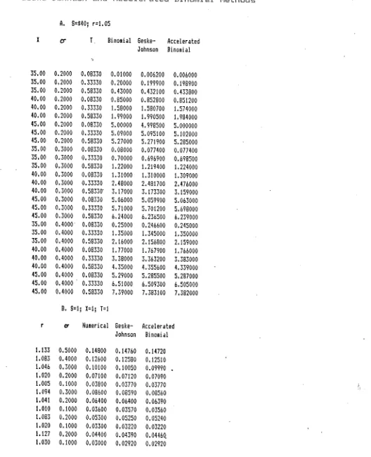
we refer first to Table I.~ wher’e three sets of Americ:an
option values, for" the data -originally given by Cox and
Rubinstein [4] and F’arkinson [8] are shov.~n, These three-sets
of values are based on., respectively., the unmodified binomial
with 150 periods or Parkinson’~s numeric:al apprc, ac:h; the
Geske-Johnson ’~ analytic"~ method us i ~’~g a four point
extrapolation; and the ac:celerat.ed binomial metlnod presented
here., using a three point extrapolation over a 150 period
model. All three sets o’f values agree very closely. The
largest error in the accelerated binomial method is of the
order of one an~ a half cents coci~pared with the b.ino~~ial or
numeric’al value. Clearly a four point extrapolation would be
more accurate, What is most str’iking about the accelerated
binomial method., ho~ever".~ is the reduction it brings about in
the amount of computation required, The unmodified binomial
method reqL!ires the calc.Ltlation of (N+I)e node values, which.~
for N=I50.~ is 22801. The accelerated binomia!.~ on the other
hand, calls for only 4.N + I0 calculations - 610 for a 150
period model. Thus tlne accelerated binomial is very much
faster than the bin~.~mia], method, redu.r..ing the number’ of node
value calculations by 97 per cent. A second source of
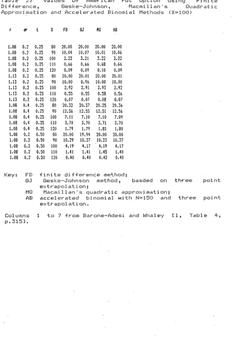
comparison will be found in Table 2., ~hich shows put option
values calculated using the accelerated binomial together
with values obtained using three other methods - the finite
difference method.~ the Geske-Johnson method and Mar...mil’lan~s
9
methods against the finite dif’ference values it c:an be seen
that there is little to choose between them, although the
accelerated binomial is, i’f any’thing marginally more a~c~ur’ate
than either the Geske-O’ohnson model (which is here computed
using a three point extrapolation) or" Ma(;millan’~s. A similar
conclusion is r’ea~.~hed i’f we compare the a(.~celerated binomial
values in the present ]"able 1 with those given by Macmillan
[9, pp. 131-132] for" the same data using his own method.
[ TABLES I AND 2 HERE ]
V Cc}nc).L~sion
The only previous attempt to investigate t.he applicat, ion of
convergence ac.celeration techniques to the binomial option
pricing model is contained .in a paper by Omberg [7] . His
approach diffe1’~s from the present one insofar as he sought to
find a means by which to accelerate the convergence of a
sequence of binomial option models with increasing N (rather
than, as in the approach used here, seeking to accelerate the
convergence of a particular binomial model with fi,~,ed N) .
However, such a sequenc.e converges in an oscillating, rather’
than uniform, manner, and On, berg showed that it was
impossible to select the parameters of the binomial model in
such a way as to ensure uniform convergen(~e. Nevertheless,
Omberg [7, p.464.] notes that, if convergence acceleration
could be applied to the binomial, then "binomial-pricing
models might prove to be considerably more eff~.¢:ient than
compound option models".
both the binomial and ...~ .i ... ~,,~ one ,, ... ,
it is mt.lGh faster- than the unmodif led binomial, suggesting
that it might prove to b(--~ more efficient than other numeri(al
methods (such as finite differonce methods) not only for
valuing a small number of optionss, but also for valuing a
large number. On the other hand, the accelerat.ed binomial,
viewed as an approYimation to the Geske-Johnson model,
removes the need to evaluate multivar’iate normal integrals of
up to order three or four (in a four point extrapolation) - a
cemputational].y time consuming task. =-’ That this is the main
disadvantage of the Gesl.::e-Johnson method has been recognised
by a number of authors, including Barone-Adesi and Whaley
[I], Omberg [7] and also Selby and Hodges [10] who have
demonstrated a means by which the integral e’~aluation prob].em
c::an be ...~o more manageab],e proportiorlsed u(... eu . ]"he approach
outlined here, however, i’~ likely to prove i:ar’ more
convenient and accessible even than a 8eske-Johnson model
incorporating Selby and Hodges’~ modifications.
Sin~e the binomial itself is an approximation to the true
option value, our application of the Richardson e,vtr’apolation
technique yields an approximation to an approyimation.
Nevertheles.=i, this can be made as accurate as one desires,
first by choosing a sufficiently large value for" N, and,
secondly, by e~-’trapolating from a greater number of eyercise
points. Clearly, however’, our choice of the conventional
value of N (15(:)) and of a simple three point ei.(trapolation
yields results which are sufficiently accurate for most
ii
here is a modific:at’i.c~n to the binc~mial, it reta.ins.; all the
fleY, ibility of the latter. Thus the ac.celerated bin~3mial can
be used tc~ value all t.he variety (.~f options (on fclreign
e;.’change, c:ommc, dities, ’futures, and so on) for whi(:h the
FOOTNOTES
I. By which we mean, of c:c)urse, the prclbability within the binomial model implied by the risk neutrality assumpt, ion.
2. As with the sequence F’(n), this means that F" (n) does. not converge uniformly to its limit. In discussing the Geske-Johnson model Omberg [7, pp 463-464] has s~.f~ge,-::,ted that unifor’m c:onvergenc:e of the sequence of P(n) would be desirable on the c]rounds that this would ensure that the convergence acceleration technique per’forms as int.ended. For’ both the sequences P(n) and F’’~ (n) this could be accomplished by ensuring that each term in the sequer~ce permits early exercise at every instant (cir’ period, in the case. of F" (n)) at which exercise was permitted in forming ear].ier terms. Thus, the term F:’(3) in the Gesk.e-Johnson sequence would be amended to permit eyer’cise at T, 3T/4, 2T/4 and T/4 - and. analogously for P’~ (3). In what follows, however, we retain the original spe~.i’fic.ations of the terms of P and P’~.
*_%
APPEND I X
Uniform [imnvergence is defined by Dini"s theorem. In our
case4 to show that the sequenc.e of functions F:’~(ED (a=O ...
N) converges uniformly we need only to demonstrate that, for
all S, P~(S)~ P~_..~. (S) .
Wr’ite F’~-i (S) as
n
}] (p/q) J ((l-p) lq) ~’"J Vj
j =0
(n-9
= Ii ,~. j / (p/q) J ((l-.-p) /q) ~-±-J V j,.., (l-p)/q
j =0
n-I (n-- I~
¯+ Z \j-lJ(p/q) j-I ((l-p)/q),-,-J V3,., p/q j=l
Write F’~ (c,) as
n-I (n-l)
Z j (p/q) J ((1-p)/q),",-t-J j =0
Vj ~,~-. ~.
(al)
(a~.
Since for all Vj~,
Vj.~,_z >/ Vj+±.,.,(p/q) + Vjr, (l-p)/q
a2 is ~/
n-I (n~. i)
"£ (p/q) J ((l-p)/q) ~--l-j j =0
[Vj+±.,..,(p/q) + Vj,.., (1-p)/q]
C-9
= Z j (plq) J ((l--p) lq) ~-’i-J Vj~ (l-p) lq
j =0
n-I (n- 0
+ 7. j (p/q) j-i (Xl-p)/q)~-l.-j V j+l.~, j=O
plq
= 1-.., j (p/q) J ((l-p)/q) ,-.,-i-j Vj ~ (l-p)/q
j = 0
o (’n-q
+ I] j-lJ (p/q) J-~. ((l-p)/q) ~"-’J V j,.., p/q
15
i. Barone-Adesi, G. and R. E. Whaley.
Approximation o~ Amer"ic:an Option Values." 42 (June 1987) , 301-320.
’E~.fi cient Analytic
Journal o*" Finance
2. Breen, R. ’Improving the Efficiency o; the Binomial Option Pricing Model.’ unpublished working paper, 1988.
¯ - Co;.’ J C.~.’" A Ross ancl M. Rubinstein. ’Option Pricincl:
~ ~ ~ . ~ "
A Simplified Approac:h. ’ Journal o$ F’inanciaZ Economics 7
(September 1979) , .~’.~.-..:,-~.~b..:,,
4.. Cox, J.C. and M. Rubinstein. Options Markets. Cli~s, N.J. : Prentice Hall, 1985.
Engl ewood
5. Geske, R. and H. E. Johnson. ’The American Put Optior’! Valued Analytically.’ Jour1~al of Finance 34 (December 1984), 15:1. :1.-:1.524.
6. Geske, R. and K. Shastri. ’Valuation by Approximation: A Comparison o~ Alternative Option Valuation Tecl-~r~i ques. ’
Journal of Financial and Quantitative Analysis ~:.~ (Marc:h
1985) , 45-71.
I
7. Omberg, E. ’A Note on the Cor’ivergence o~ the Binomial-Pricing and Compour~d-Option Models.’ Journal o," Finance 42
(June 1987), 463-469.
8. Parkinson, M. ’Option Pricing: The American Put."
Journal of Business ~(. (January 1977), 41-36
?"he
9. Macmillan, L. W. ’Analytic Appro;.’imation for the American Pu’I: Option.’ Advances in Futures and Options Research 1
(1986) , -119-139.
TABLES
Table I: Values of American Put Option . using
Geske-Oohrlson and Ac:celerated Binomial Methods numerical
A. 8=$40; r=l.05
X ~ T Binomial Geske- Accelerated Johnson Binomial
35.00 0.2000 0.08330 0.01000 0.006200 0.006000 35.00 0.2000 0.33330 0.20000 0.199900 0.198900 35.00 0.2000 0.58330 0.43000 0.432100 0.433800 40.00 0.2000 0.08330 0.85000 0.852800 0.851200 40.00 0.2000 0.33330 1.58000 1.580700 1.574000 40.00 0.2000 0.58330 1.99000 1.990500 1.984000 45.00 0.2000 0.08330 5.00000 4.998500 5.000000 45.00 0.2000 0.33330 5.09000 5.095100 5.102000 45.00 0.2000 0.58330 5.27000 5.271900 5.285000 35.00 0.3000 0.08330 0.08000 0.077400 0.077400 35.00 0.3000 0.33330 0.70000 0.696900 0.698500 35.00 0.3000 0.58330 1.22000 1.219400 1.224000 40.00 0.3000 0.08330 1.31000 1.310000 1.309000 40.00 0.3000 0.33330 2.48000 2.481700 2.476000 40.00 0.3000 0.58330" 3.17000 3.173300 3.159000 45.00 0.3000 0.08330 5.06000 5.059900 5.063000 45.00 0.3000 0.33330 5.71000 5.701200 5.698000 45.00 0.3000 0.58330 6.24000 6.236500 6.239000 35.00 0.4000 0.08330 0.25000 0.246600 0.245000 35.00 0.4000 0.33330 1.35000 1.345000 1.350000 35.00 0.4000 0.58330 2.16000 2.156800 2.159000 40.00 0.4000 0.08330 1.77000 1.767900 1.766000 40.00 0.4000 0.33330 3.38000 3.363200 3.383000 40.00 0.4000 0.58330 4.35000 4.355600 4.339000 45.00 0.4000 0.08330 5.29000 5.285500 5.287000 45.00 0.4000 0.33330 6.51000 6.50%00 6.505000 45.00 0.4000 0.58330 7.39000 7.383100 7.382000
B. 8=I; X=I; T=I
r Numerical Geske- Accelerated
Johnson Binomial
17
Notes to Table I:
For the binomial and accelerated binomial , N=I50.
Table 2: Values o; American Put Option using Finite
DiTTer’enc:e, Geske-Johnson, Macmi I i an ’ s Quadratic Approxiri,ar~’ien and Accelerated Binomial Methods (X=IO0)
r o- t S FD GJ MO AB
1.08 0.2 0.25 80 20.00 20.00 20.00 20.00 1.08 0.2 0.25 90 10.04 10.07 I0.01 10.06 1,08 0.2 0.25 I00 3.22 3.21 3.22 3.22 I.OB 0.2 0.25 110 0.66 0.66 0.6B 0.66 l,OB 0,2 0,25 120 0,09 0,09 0, I0 0,09 1,13 0,2 0,25 80 20,00 20.01 20.00 20,01 1.13 0.2 0.25 90 I0.00 0.96 I0.00 I0.00 1,13 0.2 0,25 I00 2,92 2,91 2,93 2,92 1,13 0,2 0,25 II0 0,55 0,55 0,5B 0,56 1.13 0.2 0.25 120 0.07 0.07 0.08 0.07 l,OB 0.4 0,25 80 20,32 20,37 20.25 20,36 1,08 0,4 0,25 90 12,56 12.55 1.2,51 12,56 l.OB 0.4 0.25 I00 7.11 7.10 7.10 7.09 1.08 0.4 0.25 II0 3.70 3.70 3.71 3.70 1.08 0.4 0.25 120 1.79 1.79 1.81 1.80 I,OB 0,2 0,50 80 20,00 19,94 20,00 20,00 1,08 0,2 0,50 90 10,29 10,37 10,23 10,37 1,0B 0,2 0,50 100 4,19 4.17 4,19 4,17 l,OB 0,2 0,50 II0 1,41 1,41 1,45 1,40 l.OB 0.2 0.50 120 0.40 0.40 0.42 0.40
Key: FD Tinite diTference method;
GJ Geske-Johnson method, basded on
extrapol ati on;
MQ Macmillan’s quadratic approximation;
AB accelerated binomial with N=150 and
extrapolation.
Col umns p.315].
1 to 7 from Barone-Adesi and Whaley
three point
three point