Entanglement of multipartite quantum states and the generalized quantum search

(1)

Entanglement of Multipartite Quantum States

and the Generalized Quantum Search

Thesis by

Robert

M. Gingrich

In Partial Fulfillment of the Requirements for the Degree of

Doctor of Philosophy

California Institute of Technology Pasadena, California

2002

(2)

COPYRlGHT

©

(3)

ACKNOWLEDGEMENTS

III

Acknowledgements

(4)

ABSTRACT IV

Abstract

In chapter 2 vanous parameterizations for the orbits under local unitary transformations of three-qubit pure states are analyzed. It is shown that the entanglement monotones of any multipartite pure state uniquely determine the orbit of that state. It follows that there must be an entanglement monotone for three-qu bit pure states which depends on the Kempe invariant defined in [1]. A form for such an entanglement monotone is proposed. A theorem is proved that significantly reduces the number of entanglement monotones that must be looked at to find the max.imal probability of transforming one multipartite state to another.

In chapter 3 Grover's unstructured quantum search algorithm is generalized to use an arbitrary starting superposition and an arbitrary unitary matrix. A formulafm the probability of the generalized Grover's algorithm succeeding after n iterations is derived. This fmmula is used to determine the optimal strategy for using the unstructured quantum search algorithm. The speedup obtained illustrates that a hybrid use of quantum computing and classical computing techniques can yield a performance that is better than either alone. The analysis is extended to the case of a society of k quantum searches acting in parallel.

(5)

CONTENTS v

r

.

(6)

LIST OF FIGURES

List of Figures

3.1 Plot of the probability of success of Grover's algorithm after n iterations of amplitude amplification when there are '" solutions amongst N

=

64 possibilities. White regions correspond to prob-ability 1, black regions correspond to probability O. Note that

VI

the success probability is periodic in the number of amplitude amplification iterations for a fixed number of solutions . . . .. ". 31 3.2 Plot of the optimal number of iterations to use in k-parallel

(7)

CHAPTER 1. INTRODUCTION 1

Chapter 1 Introd uction

At this point in history quantum mechanics is the best description of nature that exists. No repeatable experiment has ever contradicted it, yet it is still not very well understood. Compared to classical mechanics, the principles of quantum mechanics are less intuitive and the mathematics is often more difficult. Nevertheless, if one wants to know what is possible in nature, one must look at the true quantum mechanical description, not the approximation of classical mechanics.

In the last 30 years computers and digital information have become impor-tant in our society. This has been made possible by, among other advances, our understanding of computation, algorithms, information compression and error correction. These areas of study have, until recently, been based solely on classi-cal principles and intuition. In the last decade is has been shown that by looking at the true quantum mechanical description new phenomena are possible (e. g., Shor's algorithm, teleportation, Grover's algorithm, quantum error correction). This has led to the studies of quantum computation and quantum information theory.

(8)

entan-CHAPTER 1. INTRODUCTION 2

glement. These systems are said to be represented by a separable state. The correlations between the subsystems of an entangled (i. e., non-separable) state cannot be fully explained by classical physics. The first step in understanding what new phenomena are possible with quantum information is to find out what states are non-classical. In chapter 4 a criterion for detecting separability called the "reduction criterion" is investigated. This criterion is shown to be equiv-alent to the already known Peres criterion in 2 X N systems and to be helpful in the calculation of the entanglement of formation (a particular measure of entanglement) for 2 x 2 systems.

Entanglement between more than two subsystems is more complicated and hence less well understood than the entanglement between two subsystems. This problem is addressed in chapter 2. A framework for characterizing the set of all measures of entanglement, called entanglement monotones, is proposed. This framework is used to show that there are some important yet undiscovered entanglement monotones for systems with 3 two-dimensional subsystems. Some properties of these entanglement monotones are derived and an explicit form is proposed for one of them.

(9)

CHAPTER 1. INTRODUCTION 3

In chapter 3 an equation for the computation time of grover's algorithm with

(10)

CHAPTER 2. PROPERTIES OF ENTANGLEMENT MONOTONES 4

Chapter 2 Properties of Entanglement

Monotones

2.1 Introduction

Entanglement is at the heart of the studies of quantum computation and quan-tum information theory. It is what separates these studies from their classical

counterparts. If we are to understand what new phenomena occur when we look at the true quantum mechanical description of nature as opposed to the

approximations of classical mechanics, then we must understand how the quan -tum mechanical description differs from the classical description. Entanglement is a measure of this difference. While entanglement between two parties is quite well understood [3] [4] [5] [6], the entanglement within a quantum algorithm or in a state shared between many parties involves multipartite entanglement

which is just beginning to be understood [7] [8] [9].

(11)

Communication (LOCe). For two part systems this problem is solved, or at

least reduced to the problem of finding the eigenvalues of a hermitian matrix,

by [5] [6]. For a N x M pure state the Schmidt decomposition tells us we can

write

(2.1)

;=1

w here the

AT

are in increasing order,

Ei

AT

= 1, the

1

i) and

1

i') are an orthonor-mal set of vectors in space A and B respectively, and n

=

min(N, M). If we define

k

Edl-,p))

=

I:>-T

k = 1, .. . ,n-1 (2.2)

then the highest attainable probability of transforming

l

-,p)

to

1 4»,

P(I-,p) -t

1 4»),

is given by [6]

.

Edl-,p))

P(I-,p) -t

1 4»)

=

n;:n

Ek (14))) (2.3) The proof of this theorem is constructive so we can actually write down the

transformation that gives us

1 4»

from

l-,p).

For pure states of more than two

parts no such nice theorem is known. The question of whether two three-qubit

pure states can be transformed into each other with non-zero probability by

LOCC has been solved by Diir et al. [10] but just getting a reasonable upper

bound on that probability when it is a non-zero is unsolved. In this paper I

attempt to make some progress towards solving this problem for three-qubit

pure states and hopefully shed some light on how we might solve it for larger

dimensional spaces and more parts.

One way to find P(I-,p) -t

14»)

is to look at the entanglement monotones E(I-,p)) for the two states. For the duration of the paper "state" will refer to a pure state unless explicitly called a mixed state. An entanglement monotone,

EM, is defined as a function that goes from states to positive real numbers and

does not increase under LOCC. As a convention the value of any EM for a

(12)

CHAPTER 2. PROPERTIES OF ENTANGLEMENT MONOTONES 6

of parts, the following theorem holds [11):

( ') . E (p)

p p -+ P =

min

E (pi) (2.4)

where the minimization is taken over the set of all EMs [11). This can be seen by considering P(p -+ pi) as an EM for p. The problem is that this minimization is difficult to take since there is no known way to characterize all the entanglement monotones for multipartite states. We would like a "minimal set" of EMs similar

to the Ek for the bipartite case in order to take the minimization.

The situation for three or more parts is somewhat different than for bipar-tite pure states. Firstly, generic M x M bipartite states have a stabilizer (i. e., the set of unitaries that takes a state to itself) of dimension IvI - 1 isomor-phic to U(1)0M_- 1 _{while pure states with more parts generically}_hav_e_{a discrete}

stabilizer. States whose parts are not of the same dimension may ha.vp. largp.r

stabilizers but bipartite states are the only ones that always have a co ntinu-ous stabilizer. Secondly, the generalized Schmidt decomposition, however you

choose to generalize it [12) [13), has complex coefficients for pure states with three or more parts. This implies that generically these states are not local uni-tarily equivalent to their complex conjugate states (i. e., the state with each of its coefficients complex conjugated). Also, for bipartite pure states all the local unitary (L U) invariants can be calculated from the eigenvalues of the reduced density matrices but this does not hold for more parts. I will go into more detail about LU invariants in the next section.

The structure of the paper is as follows: in section 2.2 the interconvertibil

(13)

algebraically independent of the known EMs. A form for this EM is proposed

and studied. Section 2.4 discusses other monotones that must exist and their

properties. Lastly, in section 2.5 a theorem is proved that significantly reduces

the number of EMs that must be minimized over to get P(p -+ pi) of equation

(2.4) .

2.2 Decompositions and Invariants ofThree-Qubit

Pure States

Let

l

..p)

be a multipartite state in llJ ® 1£2 ... ®

ll

n and let

Ai

')

:

1£. -+ 1£; be

Krauss operators for an operation on the hilbert space 1£. with

Lk Ai

'

)

t

Ai

')

=

I. and Ii is the identity acting on 1£ •. A (non-increasing) EM is a real valued

function E

(

I

..p»

such that

(

(')

)

E

(I..p»

::::

_{2(Pk E}

h

® ... ®

A~

... ®

In

l

..p

)

_(2.5)

for any state

l

..p),

operation

A

t),

and space i where

(2.6)

This definition for pure states is taken from the definition for a general state in

[11]. One can always transform a state into product states and a product state

cannot be transformed into anything but another product state so the value of

an EM for a product state is chosen to be zero and all other states must have

a non-negative value for the EM. Since Aii) can be a unitary operator or the

inverse of that operator, equation (2.5) implies that all EMs must be invariant

under LU. Hence, a first step to understanding the EMs is to look at the LU

invariants that parameterize the set of orbits.

There are many ways to find LU invariants for three-qubit states [14] [13]

(14)

spaces, but for now I will concentrate on the three-qubit case. The three sets

of invariants I will look at in this section are the polynomial invariants [14],

what I will call the diagonalization decomposition [13] and what I will call the

maximization decomposition [12].

2.2.1 The Polynomial Invariants

A general polynomial invariant P",T

(11/»)

for a state of the form

1

I

1/»

=

L

tijklijk) (2.7)

i)j,k=O

is written as

where (J" and T are permutations on n elements, repeated indices are summed

and

t

stands for the complex conjugate of t [14]. If one applies a unitary to

any of the qubits in

I

1/»

and explicitly writes out P",T

(

1 1/»)

again, it becomes apparent that P",T

(1

1/»

)

is invariant. Of course, any polynomial in terms of the

polynomial invariants P",T (11/») is another polynomial invariant. In fact, it can

be shown that all the polynomial invariants are of this form.

We know from [12] that generic three-qubit states have a discrete stabilizer

so the number of independent polynomial invariants is given by

dim [C2 0 C2 0 C2] - 3 dim[SU(2)]-dim[U(1)]-1 = 5 (2.9)

where the last - 1 is due to the fact that we are using normalized states. The

five independent continuous invariants are

It

Pe,(12)

(15)

14 P(123),(132)

15

12:

tidlkl ti2j2k'l ti3j3k3 ti.d<Jk4

X €i 1 i2 fi3i4 fjd2 fj3j" €k1i3 Ek2i412 (2.10)

where EOO

=

En

=

0, and EOI

=

- flO

=

1 and again repeated indices are summed. 14 is the Kempe invariant referred to in the abstract. If one writes out

Is

and uses the identity f;jfr•

=

elirelj, - eli.eljr, it can be shown that

Is

is just the sum and difference of 64 polynomials of the form in equation (2.8). With one more discrete invariant,

h

=

sign[Im[ P(34)(56),(13524)]] , (2.11)

the LV orbit of a three-qubit state is determined uniquely [13] [18]. I will define sign[x] as 1 for non-negative numbers and -1 otherwise. The polynomial invariants have the advantage of being easy to compute for any state and the four previously known independent EMs [7] are the following simple functions of

h,

12 , fa and

Is

T(AB)C 2(1 - h) T(AC)B 2(1 - 12) T(BC)A 2(1 - fa)

TABC

=

20s.

(2.12)

2.

2 T

he Diag

o

na

l

izat

io

n

D

ecompos

i

tion

The diagonalization decomposition, DD, introduced by Acin et al. [13] is ac

(16)

to get rid of as many phases as possible. What is left is a state of the form

I-rPDD) =

50

1000) +

$I

ei<P1100)

+521 101 ) + VfI31110) + vfii41111) (2.13)

where J.li

2:

0, J.!o + J.!1 + J.!2 + J.!3 + J.l4 = 1 and 0 ::; ¢ ::; 1r. Note that generically there are two unit aries that will make To singular, but it can be shown that only one will lead to ¢ between 0 and 1r. If there is another solution, with ¢ between 1r and 21r exclusive, it is referred to as the dual state of I-rPDD)' Some nice properties of DD are that there is a 1 to 1 correspondence with the orbits and there are a set of invertible functions between the parameters of the decomposition and the set of polynomial invariants given above. Namely,

h

1 - 2J.!O(J.!2

+

J.!4) - 2~

I2 1 - 2J.!O(J.!3

+

J.!4) - 2~

Ia 1 - 2J.!O(J.!2

+

J.!3

+

J.!4)

I4 1 - 3[(J.!2

+

J.!3)(J.!O - J.!4)

+

J.!4(1 - J.!4)

-J.!2J.!3J.!O

+

(1 - J.!o)(~ - J.!1J.!4)]

Is

4J.!6J.1~

h

= sign[sin( ¢)

J.!

6V

J.!1J.!2J.!3J.!4

x(~ - J.!4(1- 2J.!o

+

J.!J) - J.!2J.!3)] (2.14)

where ~

=

J.!1J.!4

+

J.!2J.!3 - 2

_V

J.!1J.!2J.!3J.!4 cos(¢) and if we define

h

=

~

( 1 -

h

- h

+

Ia - 2VIs)

J2

=

~

(1 -

h

+

h

-

Ia - 2VIs)

Ja

~

(1

+

II -

h -

I3 - 2VIs)

J4

=

VIs

J5

=

~ (~-

h

- h -

Ia

+

iI4 - 2VIs) (2.15)

(17)

CHAPTER 2. PROPERTIES OF ENTANGLEMENT MONOTONES 11

then the coefficients are given by

=

J4

+ J5

±VT

2(JI

+ J

4 )

Ji

-::±' i=2,3,4

J.'o

1 _ ,,± _

h

+

h

+

J4

,..0 ±

J.'o J.'tJ.';

+

J.'~J.'t

-!t

2JJ.'tJ.'~J.'tJ.';

h

sign

[JJ.'tJ.'~J.'tJ.';[JI

- J2h

-J4

(h +

h

+

J4 - (J.'~)2)]] (2.16)

where Y = (J4+J5)2_4(JI +J4)(h+J4)(h+J4)

2:

O. The

+

and - solutions for the coefficients correspond to I'liDD} and its dual state. The inversion of the equations for Ii was done independently in [18]. Note that their definition of 14 is different from the one in this thesis.

Another nice property of the DD is that we can perform an arbitrary mea-surement on it in space A and stay in the DD form. Since any measurement

can be broken into a series of two outcome measurements [19], we can look at the two outcome measurement Al and A2 where AI Al

+

A1A2

=

I. Using the

singular value decomposition, we can write Ai = UiDi V where V does not de-pend on i because the two positive hermitian operators AI Al and A1A2 sum to the identity and therefore must be simultaneously diagonalizable. The diagonal matrices, Di , can be written as

(2.17)

(18)

form

(2.18)

where

.pI

and .pz are real numbers, commute with the Di matrices so the most general V can be written as

(2.19)

where 0

<

a

<

1 and

e

is real. If we choose

1 [ yo _x~eiO

1 U

I

V"Y

x~e-iO ya

'Y

y2 a2

+

x2(1 _ (2) (2.20)

and similarly for U2 with (x, y) replaced with

(-J1="X2

,

vIl7)

,

then in going from I.pDD) to AII.pDD) the DD coefficients undergo the following transfo rma-tions:

-+

x Zy2pO Po -

-'Y

PI

-+

~

ICi

O

(

x

Z - y2)aJpo(l - ( 2)

+

ei4>

'Yv1'

lf

Pi

-+

Pi"! i = 2,3,4

<P

-+

arg [e-iO (x2 - y2)aJ Po(1 - ( 2)

+

ei

4>'Y'Ji:ll]

(2.21)

and again similarly for Azl.pDD). Things become more complicated when <p

(19)

2.2.3 The

Maximization Decomposition

The Maximization Decomposition [12], MD, has a somewhat different way of decomposing the three qubit states. First we find the states, I¢A), I¢B) and I¢c) each defined up to an overall phase, that maximize

(2.22) and apply a unitary such that I¢A)I¢B)I¢c) becomes 1000). Defining 11), up to an overall phase, as the vector perpendicular to 10), then the derivative of 9 along 11) at the point 1000),

11m . g(IO)

+

Ell), 10), 10» - g(IO), 10), 10»

€-tO <:

= 2Re [(,p1100)(0001,p)] (2.23)

must be zero because g(IO), 10), 10» is a maximum. Since we still have phase freedom in 10) and 11) this implies that (,pll00) = a and similarly for (,plaID) and (,p1001). Using the remaining phase freedom in the choice of 10) and 11), we can eliminate all but one phase leaving us with

I,pMD) = aei<PIOOO)

+ blOll)

+

c1101)

+

dlllO)

+

filII) (2.24) where a2

+

b2

+

c2

₊

_d2

₊

_f₂₌_1,₀

:s

_¢

:s

_27T,₀

:s

_a,_b,_c,_d,_f _and_b_,_c_,_d,_f

:s

a. Note that g(lOA)' lOB), lac» = a2 _{Unfortunately,}_the_p_arameters_as_they are given above are not in 1 to 1 correspondence with the orbits. While the decomposition is generically unique, there are choices of the parameters within the given ranges that are not the result of the decomposition. For example, states with a2 = ~

+

€, b2 = c2 = d2 = f2 = ~ - ~ and any choice of ¢ have

(2.25)

for €

:s

0.014. Hence, these choices of the parameters are not a result of the

(20)

A nice property of the MD is that is it symmetric in particle exchange.

Exchanging the particles is equivalent to exchanging b, c and d. This makes the

permutation properties of the polynomial invariants easier to see when written

in terms of the MD coefficients. They take the following form:

It

1 - 2 ((a 2

+

d2)(b2

+

c2)

+

a2 f2)

h

1-2 ((a 2

+

c2)(b2

+

d2)

+

a2 f2)

fa

1 - 2 ((a 2

+

b2)(c2

+

d2)

+

a2 f2)

I. 1 - 3(a2(1 - a2) - Wc2

+

b2d2

+

c2d2)(1 - 2a2)

_2b2_c2_d2_- _2abcdf₂_cos(q,))

15 a21 af2

+

4bcdei<P12

Is

sign[abcdf2 sin(q,)(a2(1 - 2a2)(1-2a2 - f2)

_4b 2c2d2 - 2abcdf2 cos(q,))]. (2.26)

It is apparent from these equations that It, h and

fa

are symmetric in permuta-tions of particles AB, AC and BC respectively and 14 ,

Is

and Is are symmetric

in any permutation of the particles. Unfortunately, the equations in (2.26) are

not as easy to invert as those in (2.14). In fact, just calculating the MD co-efficients for an arbitrary state is not an easy task, as it is in the case of the polynomial invariants and the DD coefficients, since determining the unitaries

for the MD involves maximizing over a six-dimensional space with typically

many local maxima.

One more interesting fact about the MD is that 1 - a2 _is_a_non-in_creasi_ng

EM. We know this because in [17] it is shown that a function of the form

(2.27)

where rx is a kx-dimensional projector on system X = A, B, C, IS a

(21)

CHAPTER 2. PROPERTIES OF ENTANGLEMENT MONOTONES 15

independent of the T from equation (2.12) by looking at the gradient vectors of

the T, 1 - a2 and N = a2

+

b2

+

c2

+

d2

+

f2 at, for instance, the point a = 3, b, c, d,

f

= 1 and ¢ = ~. Since the gradient vectors span a six-dimensional space, 1-a2 _{cannot be writt}_en_{in terms of}_the_T_and_N._The_{problem with}_using_1-_a2

as an EM is that one needs to find the global maximum of a six-dimensional

space with many local maxima to calculate it. This is a difficult task for most

states.

2.3 Fifth Independent EM

In section 2.2 it was shown that all EMs must be invariant under LV and hence

are determined by the orbit of the state. For three qubit states this means that

EMs are a function of only the polynomial invariants, DD coefficients or MD

coefficients. In fact, this determination is unique.

Theorem 1 The set of all EMs for any multipartite pure state,

11/»,

uniquely

determine the orbit of the state.

Proof. Suppose two states

I1/»

and

I¢)

in 11.1 0 11.2· .. 0 1I.n have the same

values for the EMs but lie in different orbits. We know by using equation (2.4)

that

P(I1/» --+

I¢»

=

P(I¢) --+

11/»)

=

1 (2.28)

so

I1/»

can be transformed to

I¢)

(and vice versa) by n-party LOCC, n-LOCC,

with probability 1. Since EMs are non-increasing with any n-LOCC, they must

remam constant during the entire transformation from

I1/»

to

I¢)

(and vice

versa). Also, we know that any EM between a system X = A, B, .. . and the rest of the systems thought of as one (e. g., between Band (ACD .. .

»,

I will

call these EMs 2-EMs, is also an EM for multipartite states. This is because

(22)

of the systems, since the 2-EM is non-increasing over 2-LOCC it must also be

non-increasing over n-LOCC. In particular, the sum of the lowest k eigenvectors

of the reduced density matrices,

k

Ef(

I

'ifi

»

=

I >

T(px(I'ifi»),

(2.29)

i=l

(i. e., the 2-EMs in equation (2.2» must be EMs. So the

Ef(I'ifi»

must remain

unchanged and hence the spectrum of Px is unchanged during the transforma

-tion from

l

'ifi)

to

IqI).

In particular, a measurement on space X, given by Al and

A2, must be such that

px (

~»)

=

u

px

(

I

'ifi»

Ut (2.30)

where N is the normalization. The only way this can be satisfied is if

7Ft

is

a unitary matrix. This means that

l

'ifi)

and

IqI)

are unitarily equivalent which contradicts our original supposition. 0

Since we know there are 5 parameters that determine the orbit of a three

qubit state, then by theorem 1 there must be 5 independent, continuous EMs.

To the best of the author's knowledge, the only 4 known independent continuous

EMs that don't require a difficult maximization over a multidimensional space

are the four r EMs defined in equation (2.12). Any candidate for the fifth independent EM must depend on 14 since the r are invertible functions of 11,

12,

h

and

Is

respectively. The following function fulfills that criterion:

(2.31)

and numerical results suggest that it is an EM. After generating over 300,000

random states and applying a random operation to each of them, the inequality

in equation (2.5) was never violated by (J' ABC. Also, note that (J' ABC is

(23)

zero or perhaps just a very small measure for which" ABC is not a monotone and my numerical test didn't explore this space but there must exist some function of the polynomial invariants which is independent of the TS and is an EM. For

it to be useful in improving our upper bound for P

(

Iv»

--t 11>}), there should be pairs of states Iv>} and 11>} such that

and I have found such states numerically. The largest value of -,

" A:.:.:B:,,::C-7( I,.:,.V>;+}) _ min _T _( Iv>_}_)

"ABc(I1>}) T T(I1>})

(2.32)

(2.33)

that I found in my limited number of examples was 0.01 and I was able to find examples of states for which T (Iv>}) / T (11)}) is greater than one for all T and "ABC(IV>})/"ABc(I1>}) is less than one.

2.4 Other

EMs

and the

Discrete

Invariant

The five independent continuous EMs, T(AB)C, T(AC)B, T(BC)A' TABC and" ABC, can easily be inverted to find

h

-

Is

but to completely determine the orbit of a state we must also have an EM that will give us the value of the discrete invariant 16 • This is equivalent to finding an EM that is not the same for a

state and it complex conjugate state. Note that

Ir

,

...

Is and hence the T and

"ABC do not change when a state is conjugated, but by looking at any of the

sets of LV invariants we can see that generically a state is not LV equivalent to its conjugate. By looking at equation (2.4) we can see that this implies that there must be EMs that are not the same for the generic state and its conjugate.

(24)

the operation I'¢»~ ~ I'¢»~ and a similar one that goes down the same amount for

\~) ~ \'¢». So, EMs of the following form must exist:

{

v+v'

v± (\'¢»)

==

v

±h

==

1

(2.34) o.w.

where v and v' are functions of T(AB)C, T(AC)B, T(BC)A, T ABC and (j ABC.

Also, from [10] we know that there are two classes of three-part entangled

states (i. e., states with T(AB)C, T(AC)B, T(BC)A

>

0) that can be converted into

each other with some non-zero probability within the class and zero probability

between the classes. Namely, the GHZ-class which contains

\GHZ)

==

~

(\000)

+

\lll)) (2.35)

and has non-zero TABC and the W-class which contains

\W)

==

Js

(\001)

+

\010)

+

\100)) (2.36)

and has TABC

==

O. Looking again at equation (2.4), we see that TABC tells

us that P(\,¢>W) ~ \'¢>GHZ))

==

0 but none of the previously defined EMs tell

us that P(\'¢>GHZ) ~ \'¢>W))

==

o.

Since the only way to get P(\'¢>GHZ) ~

\'¢>W))

==

0 is to have an EM that is finite for GHZ-class states and infinite

for W-class states or zero for GHZ-class states and non-zero for W-class states,

such an EM must exist.

2.5 Finding a Minimal Set

Since T(AB)C, T(AC)B, T(BC)A, TABC, (jABC and v± determine the orbit of the

state, all other EMs must depend on them. A fairly general way to create new

EMs from known EMs is to use what I will call f-type functions.

Definition 1 A function f :

SeWn

~

W

is an f-type function if it satisfies

(25)

1. f(O)

=

0

2. if x; ~ Yi for all i = 1,2, ... n then f(i) ~ fUJ) for i,

if

£ S

3. f(pi + (1 - p)ilJ ~ pf(i) + (1 - p)f(ilJ for any i,

if

E S and 0

:S

p

:S

1.

For a set of EM, {Ed, we have

Ei(

I",»

~

pE; (

Aj;»)

+

(1 - p)E;

(~)

(2.37)

for any measurement A1 , A2 and any state

I

"').

SO, we have

f[E(I"'»]

>

f [PE (

Aj;»)

+

(1 - p)E

(~)

]

>

pf [E

(Aj;

»

)]

+

(1-p)f [E

(J;I~~)]

(2.38)

where the first inequality comes from property 2 and the second comes from

property 3. Hence, f(E1, ... , Em) is also an EM. We can show that any EM

f(E 1, ... _{,Em )}that is an f-type function of monotones E 1, _{... E m does}not

modify the upper bound on P(I"') -+ 1<1>)) given by

(I)

_1"-»

.

E;

(I

"'»

P '" -+ 'I'

:S

n:,m

E; (1<1>)) .

First for the one-dimensional case.

Lemma 1 If f(x) is an f-type function with n = 1, then

f(x) . {x } f(y) ~ mm

y,l

for any x, y £ S.

Proof.

Case 1 For x ~ y from property 2 we know f(x) ~ f(y) and hence

f(x)

>

1.

f(y)

-(2.39)

(2.40)

(26)

Case 2 For x

<

y if we choose p = ~ f [0,1), then we know from properties 1

and 3 that f(py)

2:

pf(y) and so

f(x)

>

~. 0

fry) - y (2.42)

For n dimensions we have the following theorem (proved with S. Daftuar

and D. Whitehouse).

Theorem 2 If f(x) is an f-type junction, then

fry) .

{Xi }

-(_) 2:

mm -,1

f

y Yi

i=1,2, ... n (2.43)

faT Y,

Yf

S.

Proof. Let

. {Xi}

c=mm

-Yi (2.44)

then we have

Case 1 If c

2:

1 then from property 2 fry)

2:

frY) and so

fry)

frY)

2:

L (2.45 )

Case 2 If c

<

1 then define

Xi

Zi

==

-

i== 1,2, ... n

c (2.46)

and g(T) = f(TZ). Notice that g(1') is an f-type function with n = 1 and

hence

or substituting in

f

we have

g( c)

-() >c

9 1

-fry)

f(i)

2:

c.

Using Zi

2:

Yi and property 2 we have

fry) 0

fry)

2:

c.

(2.47)

(2.48)

(27)

CHAPTER 2. PROPERTIES OF ENTANGLEMENT MONOTONES 21

For three-qubit states if we take the minimum of E(I1/»)/E(I¢» over E =

{7(AB)C, 7(AC)B, 7(BC)A' 7 ABC, (J" ABC, v±} we are actually taking the minimum

over the infinite set of all J-type functions of E. Although from theorem 1 we know that all EMs must be a function of E, it is possible that there exist EMs that are not J-type functions of E. These EMs could cause P(I1/» -+

I¢»

to be lower than the minimum of E(I1/»)/E(I¢» over E. The EM mentioned at the

end of section 2.4 is an example of such an EM.

2.6 Conclusions and Further Research

Theorem 1 along with theorem 2 implies that there should be a (not necessarily finite) minimal set of EMs, M, for which all EMs for three-qubit states or

simi-larly for any type of multipartite states are J-type functions of M. I conjecture that such a minimal set should be simple since the J-type functions seem to be a rather general way of creating EMs that are functions of other EMs. The difficult part seems to be finding the EMs that are minimal and showing that

they are minimal. Using numerical results it seems that the 7 may be minimal.

I looked at functions of the 7 that are almost but not quite J-type such as 71.01 and numerically tested whether they are EMs or not. None of them were EMs. I cannot say the same for (J" ABC and definitely not for v± since I do not have an explicit form for the v.

There is further research that may help these problems. If one could invert the equations in (2.26) to write a, b, c, d,

J

and ¢ in terms of

h,

...

,

Is that

would allow us to calculate the EM 1 - a2 _not_to_m_en_{tion find}_the_{ranges for}

and calculate the values of a, b, c, d,

J

and ¢. The EM 1 - a2 _could_{be used} to replace (J" ABC, or perhaps as an addition to E, and may prove more useful

than (J" ABC. As far as finding the minimal EMs and showing that they are

(28)

CHAPTER 2. PROPERTIES OF ENTANGLEMENT MONOTONES 22

may be useful since it allows us to look at the value of

It

,

.

..

,

h

before and

after an arbitrary measurement on an arbitrary state with far less parameters

than if we didn't take out the LU freedom. Also, it may be able to tell us

the maximal probability of transforming the general complex state I1/» to its

conjugate state

l

,p)

and this is a crucial piece of information that is needed to

calculate Vi in equation (2.34). Unfortunately, most of these tasks involve trying

to solve nontrivial equations or systems of equations with many variables which

(29)

CHAPTER 3. GENERALIZED QUANTUM SEARCH 23

Chapter 3 Generalized Quantum

Search

3.1 Introduction

The field of quantum computing has undergone a rapid growth over the past few years. Simple quantum computations have already been performed using nuclear magnetic resonance [20, 21, 22, 23, 24, 25] and nonlinear optics technologies [26, 27]. Recently, proposals for specialized devices that rely on quantum computing have also been made [28]. Such devices are far from being general-purpose computers, nevertheless, they constitute significant milestones along the road to practical quantum computing.

(30)

and an optical implimentation is given by K wiat [36]. Grover's algorithm is able to find a marked item in a virtual" database" containing N items in O(

v'Jii)

computational steps. In contrast, the best classical algorithm requires O( N /2) steps on average, and O(N) steps in the worst case. Thus Grover's algorithm

exhibits a quadratic speedup over the best classical counterpart.

Although Grover's algorithm exhibits only a polynomial speedup, it appears to be much more versatile than the other quantum algorithms. Indeed, Grover has shown how his algorithm can be used to speed up almost any other quantum

algorithm [37]. More surprisingly, even search problems that contain" structure"

in the form of correlations between the items searched over often reduce to

an exhaustive search amongst a reduced set of possibilities. Recently, it was shown how Grover's algorithm can be nested to exploit such problem structure

[32]. This is significant because NP-hard problems, which are amongst the most

challenging computational problems that arise in practice, possess exactly this

kind of problem structure.

In order to appreciate the full versatility of Grover's algorithm, it is

impor-tant to examine all the ways in which it might be generalized. For example,

whereas the original Grover algorithm was started from an equally weighted

superposition of eigenstates representing all the indices of the items in the database, a natural generalization would be to consider how it performs when started from an arbitrary initial superposition instead. This refinement is

im-portant, because if Grover's algorithm is used within some larger quantum

com-putation, it is likely to have to work on a arbitrary starting superposition rather

than a specific starting eigenstate. Similarly, the original Grover algorithm uses

a particular unitary operator, the Walsh-Hadamard operator, as the basis for a sequence of unitary operations that systematically amplifies the amplitude in the

(31)

it is now known that this is not the best choice if there is partial information

as to the likely location of the target item in the database. In such a situation

a different unitary operator is desirable [38]. Hence, it is equally important to

understand how Grover's algorithm performs when using an arbitrary unitary

operator instead of the Walsh-Hadamard operator.

Each of these refinements have been analyzed in detail separately: Biham

et al. have considered the case of an arbitrary starting superposition [39], while

Grover considered the case of an arbitrary unitary operator [38]. In this

pa-per, we present the analysis of the fully generalized Grover algorithm in which

we incorporate both of these effects simultaneously. Our goal is to determine

the exact analytic formula for the probability of the fully generalized Grover

algorithm succeeding after n iterations when there are ,> targets amongst N

candidates. Having obtained this formula, we will recover the Biham et al. and

Grover results as special cases. We will then show that the optimal strategy, on

average, for using the fully generalized Grover algorithm consists of measuring

the memory register after about 12% fewer iterations than are needed to obtain

the maximum probability of success. This result confirms a more restricted

case reported in [40]. Finally, we show how to boost the success probability and

reduce the required coherence time by running a society of k quantum searches

independently in parallel. In particular, we derive an explicit formula

connect-ing the degree of parallelism, i.e., k, to the optimal number of iterations (for

each agent in the society) that minimizes the expected search cost overall. We

(32)

CHAPTER 3. GENERALIZED QUANTUM SEARCH

26

3 .2

Grover's Algorithm

The problem we have to solve is the following. Given a function f(Xi) on a set X of input states such that

if Xi is a target element

(3.1)

otherwise

How do we find a target element by using the least number of calls to the function f(x;)? In general, there might be r target elements, in which case any one will suffice as the answer.

To solve the problem using Grover's algorithm we first form a Hilbert space with an orthonormal basis element for each input Xi EX. In this paper, we refer to the basis of input eigenstates as the measurement basis. Let N =

IX

I

be the cardinality of X. Without loss of generality, we will write the target states as Iti) (with i = 1", .r), and the non-target states as Iii) (with i = 1,···N - r). The function call is to be implemented by a unitary operator that acts as follows:

IXi)ly) -+ IXi)ly Ell f(x;) (3.2)

where Iy) is either 10) or 11). By acting on

(~

lil l;)

+

1;

k

j

Itj»)

~

(10) - 11»)

(3.3)

with this operator we construct the state

(3.4)

(33)

r

1- 2

L

lii)(iil (3.5) i=l

although we emphasize that this operation can be performed without knowing

the target states explicitly but only through the knowledge of f(x).

Next we construct the operator Q defined as

(3.6)

where la) can be thought of as the state with respect to which an "inversion"

is performed. Different choices of la) give rise to different unitary operators for

performing amplitude amplification. In the original Grover algorithm, the state

la) was chosen to be

la) = _1

L

Ix)

v'N

xEX

(3.7)

and was obtained by applying the Walsh-Hadamard operator, U, to a starting

state Is), i.e., la) = Uls). Hence, the operation 2Ia)(al-1, which Grover referred

to as "inversion about the average," is equivalent to -U I,Ut with U being the

Walsh-Hadamard operator and Is being 1 - 2Is)(sl. By knowing more about

the structure of the problem, we can choose other vectors la) that will allow us

to find a target state faster. Techniques for doing this are given in [37].

If we write out Q, we get

r N-r

Q

=

L

Iti)(ti

1-

L

Ilj )(lj

1+

2Ia)(al- 4vla)(tl (3.8)

j=l

where Ii), the normalized projection of la) onto the space of target states, is

given by

1 r

It) = -

L

(ti la) Iti)

v i=l

r

v2 =

L

I(ti laW

i=l

(34)

28

We can see from this that

Q

only acts non-trivially on the space spanned by

la) and It). We can make these vectors an orthonormal basis for this space by

using

1

II) = ~ (Ia) - vlt»)

1 - v2 (3.10)

instead of la). The vector II) is just the normalized projection of la) onto the

space of non-target states. The rest of the space (i. e., the space orthogonal to

It) and II») can be broken up into the space of target states (ST) and non-target

states (SL)' We can now write

Q

as

Q

= cos ¢ (It)(tl + 11)(11) + sin ¢ (It)(II- 11)(tl) + IT - h , (3.11)

where IT and

h

are the identity operators on (ST) and (SL), respectively, and

¢

==

arccos [1 - 2v2]. From this we can see that

Q

is just a simple rotation

matrix on the two-dimensional space spanned by II) and It), and acts trivially

on the rest of the space. The operator

Q

has been independently shown by

Jozsa [35] to be an exact rotation in the special case of one solution and with

la) given by equation (3.7).

An arbitrary starting superposition Is) for the algorithm can be written as

(3.12)

where the states 1st) and lSI) (which must have a norm less than one if the

state Is) is to be properly normalized overall) are the components of Is) in (ST)

and (Sd respectively. Also, a, fJ and b are positive real numbers. After n

applications of

Q

on an arbitrary starting superposition Is), we have

Qnl s) = (acos(n¢) +,8eib_sin(n¢) _{It)+(,8eibcos(n¢) -} _asin(n¢) _{11)+lst)+(-1)}_n_lsl).

(35)

29

If we measure this state our probability of success (i.e., measuring a target state) will be given by two terms. The first term is the squared magnitude of Qnls) projected into the space

Sr.

It is equal to (stlSt) and is unchanged by Q. The second term is the squared magnitude of the component of It) which is given by

g(n)

==

l(tIQnls)12

= \ 0: cost n,p)

+

,8eib sin( n,p) \2

=

a't{3'

+

"';{3'

cos(2n,p)

+ 0:,8 cos

(b) sin(2n,p)

=

a't{3'

-

~ \0:2

₊

,62e2ib \ cos(2n,p

+

,p)

(3.14)

where

,p

==

arccos

[1"C;,::.bl]

'

This is the term that is affected by Q, and is the term we wish to maximize. The probability of success after n iterations of

Q

acting on Is) is thus

p(n, I', N)

=

(StISt)

+

g(n). (3.15)

Assuming that n is continuous (an assumption that we will justify shortly), the maxima of g(n), and hence the maxima of the probability of success of Grover's algorithm, are given by the following:

-,p

+

(1

+

2j)rr

nj

=

2,p j = 0,1,2, . (3.16)

The value of g(n) at these maxima is given by

(3.17)

In practice, the optimal n must be an integer and typically the n/s are not integers. However, since g(n) can be written as

(36)

around nj and most interesting problems will have v

«

1 and hence ¢ ~ 2v

«

1,

simply rounding nj to the nearest integer will not significantly change the final

probability of success. So, we have

( ) a2+/32 112 /322ibl ( I ) 0(2)

P n max , r, N = 2

+"2

a

+

e

+

St St - v (3.19)

as the probability of measuring a target state after n max applications of Q.

3.3 Recovering the Special Cases

As a check on our fully generalized formula for the probability of success after

n iterations, we attempt to recover the corresponding formulae obtained in the

analyses of Biham et al. (for a fixed unitary operator and an arbitrary starting

superposition) [39] and Grover (for an arbitrary unitary operator and a fixed

starting superposition) [38].

In the case of Biham et aI., the starting state is arbitrary, but the averaging

state I a) is given by

1

la)= -

L

Ix).

VN

xE-l'

(3.20)

In this case

v -_-YNrr

It)

="*

I::~=1

Iti) (3.21)

II) =

v'~-r I::;:~r I

ii)'

In the analysis of [39] they use /,;(0) and /(0) to represent the average amplitudes,

in Is), of the target and non-target states respectively, and (Tk and (Tl to represent

the standard deviations of those amplitudes. With some algebra one can see

(37)

60

50

ui'

40

r::

o

'M -I-l

::l

'b

30

Ul

o

Z

20

10

1 2 3 4

No,

iterations, n

31

[image:37.532.92.418.153.470.2]

5

Figure 3,1: Plot of the probability of success of Grover's algorithm after n iter

-ations of amplitude amplification when there are " solutions amongst N = 64

possibilities. White regions correspond to probability 1, black regions corre

-spond to probability 0, Note that the success probability is periodic in the

(38)

a -+ k(O)yIr

f3eib _-+₁₍₀₎_'"_N_- _r (stlst) -+ rO"~

(stlsl) -+ (N - r)O"l

(3.22)

¢; -+w

1j; -+ 2Re[c/>]

n -+t

no -+T.

By substituting these relationships into equations (3.14), (3.16), and (3.19), one reproduces the results of [39].

The second special case, in which la) (with respect to which inversion is done) is an unknown normalized vector, while Is) is given by

Is)

=

la)

=

~Il)

+

vlt) (3.23)

was considered by Grover. Hence, a

=

v, f3

=

v'f=V2

and b

=

O. Also,

1st)

=

lSI)

=

O. These substitutions lead to 1j;

=

¢;. Plugging this into equations (3.16) and (3.19), we get

(3.24)

and

(3.25) which agree with the results of [38]. If we examine equation (3.15) in this case,

we get

p(n)

=

1- cos«l

+

2n)¢;)

=

sin2 _«1

+

_2n)_¢;/₂₎

(39)

CHAPTER 3. GENERALIZED QUANTUM SEARCH 33

as the probability of measuring a target state after n iterations of Q.

3.4 Application of the Formula for

p(n)

Next, we show how to apply our analytic formula for the probability of success

after n iterations, P(n), to slightly speed up the quantum unstructured search

algorithm. Although the speedup we obtain is not dramatic, it is worth making

the point that it is possible at all as Zalka has proved, correctly, that Grover's

algorithm is exactly optimal [41]. Many people have assumed, therefore, that

it is impossible to beat Grover's algorithm. However, by combining techniques

of quantum computing with those of classical computing, we show that it is

possible to do a little bit better than Grover's algorithm on average. The result

we report was apparently discovered previously by Boyer et al. [40] and later

by Zalka [42] in the case where la) is a uniform superposition [as in equation

(3.7)]. It is shown here to persist for the more general case when Is) is arbitrary

but equal to la) which is the case treated in [38].

We consider a punctuated quantum search algorithm that works as follows:

Algorithm: Punctuated Quantum Search

1. Run the quantum search algorithm for n iterations.

2. Read the memory register.

3. If the result is a target state halt; else, reset the register to the starting

superposition and return to step 1.

The average time, Tavg(n), it will take to find a target state if we stop the

(40)

Tavg(n) = L~l (1-p(n))i-l p(n) in

=pf,;-J

(3.27)

_ 2n

- l- cos[(1+2n)¢I'

We can find the optimal strategy, i.e., the best number of iterations to use before

we attempt to measure the register, by minimizing the expected running time

Tavg. To do this, we set the derivative of Tavg to zero and solve for n = nopt:

oTavg 2 - 2 cos[(l

+

2n)¢]- 4n¢ sin[(l

+

2n)¢]

- - = 2 =0.

on (1 - cos[(l

+

2n)¢]) (3.28)

Typically, n will be much larger than one, so we can make the approximation

(1

+

2n)!::: n¢

==

x, so that we obtain

1 - cos 2x = 2x sin 2x

2 sin 2 _x ₌_{4x sin x cos x} _(3.29)

2x = tanx.

which gives Xopt = 1.1656 as the lowest positive solution. This solution

corre-sponds to the minimum of the function. Hence the optimal value of n is

Xopt 1.1656

nopt :::

T

= - -¢-. (3.30)

This value of n gives a probability of success of

p( nop,) = sin2 Xopt = 0.8446 (3.31)

at each measurement, and corresponds to an average number of iterations of

1 Xopt

Tavg(n op,) ::: A. . 2

'+' SIn Xopt

1.3801

¢ (3.32)

This must be compared to 2rr¢ = 1.5;08 iterations if we run Grover's algorithm

until the probability is maximal. Thus, we get a 12% reduction of the average

(41)

CHAPTER 3. GENERALIZED QUANTUM SEARCH 35

It is interesting to note that, if we restrict the analysis some more to the

case where la) is a uniform superposition and where there is only one target

state, then we have ¢ = 2/VN, so that Tavg(nopt) ~ 0.6900VN. This is faster

than the lower bounds in [43], [44], [40], and [41], but we are using a somewhat

different model. They are looking at the minimum time it would take without

measuring to find a solution with certainty up to errors from rounding n max

to the nearest integer. Instead, the model we use here allows for punctuated

measurements and resets of the quantum search algorithm. Nevertheless, the

punctuated quantum search algorithm is faster on average. Note that we have

assumed that the time it takes to measure, check if a solution was reached, and

reset the algorithm is negligible. This is reasonable as checking a solution only

requires one function call.

The punctuated quantum search algorithm has another advantage in that it

is less sensitive to decoherence. If we wait until we have the maximal probability

of measuring a target state, then we must maintain coherence for 1.5;08 steps as

compared to only 1.~55 steps for the fastest measure and restart method. This is

because we do not need to maintain coherence through the measurment stage of

this method. In fact, the punctuated search that takes the same number of steps

on average as the standard or maximal probability method (i.e., 2"'" = 1.5;08

steps) need only maintain coherence for 4"'" = 0.7:54 steps at a time. This

represents only 50% of the coherence time required in the standard Grover

method, and corresponds to waiting for a 50% probability of success and then

measuring.

3.5 k-Parallel Quantum Search

A way to speed up Grover's algorithm still further is to have a society of k

(42)

time. This is promising because the standard deviation

(J"T =

p~)

V[1- p(n)] (3.33)

in the computation time of punctuated quantum search is fairly large, and hence

having multiple searches running may give a considerable speed up.

Suppose that we know that there are exactly 7' solutions amongst N

can-didates. Given p(n, r, N), the probability of success for a single agent after

n iterations, we can boost the success probability by using k agents acting in

parallel. In particular, the probability that at least one agent, in a society of

k independent agents, succeeds after each agent has undergone n iterations is

given by

pdn) = 1 - (1-p(n))k . (3.34)

Thus, the expected cost, T~e~, of performing k-parallel quantum search is given

by

co

n

TJ~b(n)

=

j;Pk(n)(1- pdn)F-1 j n

=

Pk~n)

=

1-cos 2k

((1

+

2n)¥)

(3.35)

As in equation (3.27) we can find the value of n that minimizes the expected aTi~~(n)

cost. To find the mimimum, we find where an is equal to zero. This

derivative is given by

(k)

8Tavg(n)

8n

1 - cos2k

((1

+

2n)

¥)

(1

+

2k nq., tan

((1

+

2n)

¥ ) )

(1- cos2k

((1

+

2n)¥)f

(3.36)

For

N

«

1, i.e., when there are very few solutions amongst the items searched over, we have q.,

=

arccos(1 - ~) »J 2VJi. As before, substituting x

==

nq., :::

(1

+

2n)q.,/2 and realizing that n

»

1, we obtain

1-cos2k(X) (1

+

2kx tan(x))

(43)

In order to find the mIllunum, we thus have to solve the transcendental

equation

1 - cos2_k(x)₌_2k_{X cos2k(X) tan(x).} _(3.38)

The variable x

<

1

provided n

<

! (

j!i-

-

1).

We know that we can solve the problem with near certainty if we iterate Grover's algorithm to the maximum

probability state in

O(!kj!i-)

iterations. Hence, for a large enough number of

parallel search agents, k, there is a reasonable chance that the optimum number

of iterations, nopt('" N, k) at which the expected search cost is minimized,

sat-isfies the criterion that x

<

1. We therefore expand equation (3.37) as a series approximation in

x

about

x

= O. Actually, it appears that

x

scales as O(1/Vk),

so it tends to 0 as k tends to infinity. If we make such an expansion up to order

x2, we get

8Ti~b(n) ~

_1_ (-1

3k - 1.2 5k2 - 1.4 O(

6))

8n -

kx2

+

6 x

+

20

x

+

x .

(3.39)

A s aT(k) "a~ ( n ) . = 0 IS a secon -or er equatIOn d d . . III x , It can e so ve ana ytlcally. 2 ' b I d I '

Three of the roots are non-physical, but one corresponds to an approximation to the true minimum of Ti~1( n). Specifically, we find that Ti~b (n) is minimized

when x is given by

Xopt ::::::

5 - 15k

+

V5v

-31 - 30k

+

225k2

-3

+

15k2 (3.40)

We note that x

<

1 for all k :::: 2, so that the derivation of the optimum formula

is self-consistent. This expression for Xopt can be expanded in 1/kl /2, giving

Xopt c::: 1.1118

k;/2

+

0.0829

k;/2

+

0

(k;/2) .

(3.41)

Using 1> c::: 2v = 2J7>/N and equation (3.41), one gets the corresponding

(44)

floptimal

e

600

, ,

,

500

e

400

300

200

100

,

, ,

_,

, ,

'e"",

'e_

2 4 6

38

k

[image:44.528.99.404.113.314.2]

8

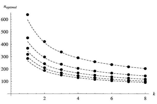
Figure 3.2: Plot of the optimal number of iterations to use in k-parallel quantum

search as a function of the degree of parallelism k for r = 1 to r = 5 solutions (top

to bottom in the figure) for the case of a database of size N = 220_._{The dashed}

curves correspond to the optima as predicted by our approximate formula for

nopt('" N, k). The points correspond to the exact optima obtained by numerical

methods.

each of k quantum searches acting independently in parallel. In Fig. 2, this

formula is shown to be in very good agreement with the exact result, obtained

by numerical optimization.

Now, if we are only interested m the scaling in Nand k of the optimal

number of iterations and expected computation time, it is enough to consider

the expansion of

&T5;~(n)

[equation (3.39)] up to order 0(1). This simply yields

Entanglement of multipartite quantum states and the generalized quantum search