A wavelet based Bayesian framework for 3D object segmentation in microscopy

A Wavelet-Based Bayesian Framework for 3D Object

Segmentation in Microscopy

Kangyu Pan

, David Corrigan

, Jens Hillebrand

, Mani Ramaswami

and Anil Kokaram

_{Electronic & Electrical Engineering Department, Trinity College Dublin, Dublin-2, Ireland.}

b

_{Institute for Neuroscience, Trinity College Dublin, Dublin-2, Ireland.}

ABSTRACT

In confocal microscopy, target objects are labeled with fluorescent markers in the living specimen, and usually appear with irregular brightness in the observed images. Also, due to the existence of out-of-focus objects in the image, the segmentation of 3-D objects in the stack of image slices captured at different depth levels of the specimen is still heavily relied on manual analysis. In this paper, a novel Bayesian model is proposed for segmenting 3-D synaptic objects from given image stack. In order to solve the irregular brightness and out-of-focus problems, the segmentation model employs a likelihood using the luminance-invariant ‘wavelet features’ of image objects in the dual-tree complex wavelet domain as well as a likelihood based on the vertical intensity profile of the image stack in 3-D. Furthermore, a smoothness ‘frame’ prior based on the a priori knowledge of the connections of the synapses is introduced to the model for enhancing the connectivity of the synapses. As a result, our model can successfully segment the in-focus target synaptic object from a 3D image stack with irregular brightness.

1. INTRODUCTION

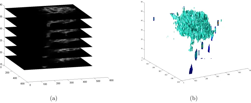
Formation of long term memory requires new protein synthesis at specific synapses of the neuron cells. The investigations of the memory formation process require the knowledge of the distribution of the proteins involved in the synthesis as well as the shapes of the synapses where the protein synthesis occurs.1, 2 The proteins have been successfully detected and abstracted from the observed images,3even with merged clustering appearance in the images, by our spot detection model4which is based on Gaussian mixture models. The goal of the algorithm proposed in this paper is segmenting the 3-D shapes of the synapses from a given stack of 2-D images (as shown in Fig.1) observed from the same living specimen but captured at at different depth by a confocal microscope.

Typically, the synapses are labelled by immunostaining with fluorescent markers in a living specimen, and a fluorescent image of the synapses is captured by confocal microscopy. However, the fluorescent markers are usually distributed unevenly over the synapses and, as a result, the synaptic objects have irregular brightness in the observed image. Furthermore, due to the physical limitation of microscope and because the synapses are 3-D objects in the living specimens, each observed image slice contains objects that are out-of-focus at the corresponding depth level. These out-of-focus objects are usually dimmer than the in-focus objects in the same image. However, since the synaptic objects have irregular brightness in the observed images, focus problem becomes even more complicated, while the object captured in-focus may have a dimmer appearance in the image but at the same time an out-of-focus focus object is brighter.

Several automatic and semi-automatic segmentation systems in confocal microscopy have been developed that apply on different tools, e.g. the K-means clustering,5_{the watershed method,}6_{the level-set framework}7_and the histogram-based method.8 _{However, in our work, due to the co-existing of irregular brightness and focusing} issue in this case, the existing techniques are unable to select the in-focus synaptic features from the given image stacks. Since the in-focus objects have sharper features in the image regardless of the local luminance, the key to resolving this problem is to consider the overall probability of the object based on both the features and intensity profile on the vertical dimension of the image stack. Therefore, we propose a segmentation model using a Bayesian framework consists of a wavelet-likelihood based on the object features and a local vertical intensity likelihood derived from the vertical intensity profile.

∗

(a) (b)

Figure 1. Sample of image stack and the result of 3D segmentation.(a) is a stack of 2-D image slices captured at different depth of a neuron specimen. (b) is a 3D illustration of the segmentation result of (a) using our model

In Section 2, we introduce the Baysian frame work and the likelihoods are described in Section 3. The wavelet-likelihood considers the luminance-invariant ‘wavelet features’ of the synaptic objects in the wavelet domain through dual-tree complex wavelet transform,9 _{and the detail of description is given in Section 3.1. In} addition, The wavelet-likelihood is co-operated with a global intensity likelihood (described in Section 3.2) in order to prevent faulty segmentation due to the existence of background noise with similar ‘wavelet features’ to the target synaptic objects. The local vertical intensity likehood measures the probability of an image object at particular image slice being in-focus while considering the propagation of intensity of that local region through the image stack. This intensity likehood term is discussed in Section 3.3. Furthermore, a priori is applied to the segmentation model in order to enhance the linkage of the connected synapses where the detail is given in Section 4. Then some segmentation results of our model are shown in Section 6.

2. BAYESIAN SEGMENTATION MODEL

Given the intensity informationIof an image stack withM image slices, the goal of our Bayesian segmentation model is to assign labels to each slice by maximizing the probability

p(b1, ...,bM|I1, ...,IM)∝p(I1, ...,IM)p(b1, ...,bM) (1)

NoteIs is the intensity matrix of image sliceswhilebs is the corresponding label field and the label (bs(x)) for a pixel (x) has the value

bs(x) =β =







1 forxin‘object0

0 forxin‘background0

In this work, we refer the pixels in the synapses as ‘object’ and all other pixels as ‘background’.

In order to make the optimization problem more tractable, we consider the optimization for each individual slice separately, Thus, we seek to maximize the posterior

p(bs|I1, ...,IM,b1, ...,bM)∝pL(I1, ...,IM|bs)pS(bs|b1, ...,bM) (2)

Furthermore, the assumption is made that the probabilities for each pixel in a given slice are independent and identically distributed (i.i.d.). Therefore, we rewrite the posterior as

p(bs|I1, ...,IM,b1, ...,bM)∝

Y

x

{pL(I1(x), ..., IM(x)|bs(x))pS(bs(x)|b1(x), ..., bs−1(x), bs+1(x), ..., bM(x))} (3)

3. LIKELIHOODS

The expression for the likelihood in Eq.(3) is factorized further into 3 separate likelihoods given by

pL(I1(x), ..., IM(x)|bs(x))∝[pW(Ws|bs(x))]

αW(β)_×[p

G(Is(x)|bs(x))]

αG(β)_×[p

V(I1(x), Is(x), ..., IM(x)|bs(x))]

αV(β) (4) The first likelihood is the wavelet-based likelihood designed to classify the image features with synaptic texture as ‘object’ regardless to the luminance of the features in the given slice. The second global intensity likelihood is intended to discriminate against regions of low-intensity in order to remove the false alarms caused by noise features with similar texture to the synaptic objects. Finally, the vertical intensity likelihood is designed to detect in-focus features and is derived from the vertical intensity profile at a given location. Furthermore, these likelihood are controlled by the weights{αW(·), αG(·), αV(·)}.

3.1 Wavelet-likelihood

Since the target synaptic object has irregular intensity in the image stack, a simple thresholding would be infeasible for the segmentation. Instead, we wish to classify pixels based on the luminance invariant texture content. The wavelet transform is ideally suited for this task since the discrete wavelet transform (DWT) decomposes an image into a luminance dependent low frequency band and a number of luminance invariant high frequency sub-bands. We propose a likelihood term using ‘wavelet features’ of image objects extracted from the high frequency sub-bands in the wavelet domain The basic idea is to use manually labelled slice to train Gaussian mixture models (GMMs) of wavelet features for both ‘object’ and ‘background’. These GMMs provide the likelihood model for all other slices in the stack.

3.1.1 Dual-tree complex wavelet transform (DTCWT)

In this work, we use the DTCWT instead of the traditional DWT to abstract the ‘wavelet features’ from the given image slices. The DTCWT is introduced by Kingsburyet al.9 which has resolved the shift-variance problem and the deficiency of frequency orientation of the classic DWT, and hence provide stable wavelet features for small offsets in synapse location.

Like the basic DWT, the DTCWT is a multi-scale transform, where each scale of the transformed image consists of one low frequency band (band) and six band-pass high frequency sub-bands (hi-bands). The lo-band is simply a down-sampled version of the input image whereas the hi-lo-bands at a given scale correspond to the response of the image to the wavelet kernel at six different orientations (±15o_,±45o_and±75o_{) in a frequency} band dictated by the scale of the wavelet. The hi-band wavelet coefficients have complex values that indicate both the magnitude and phase responses of the wavelet at the corresponding orientation.

3.1.2 Wavelet features and the Gaussian mixture model

Based on the DTCWT metric, we introduce the wavelet-likelihood that estimates the likelihood probability of each pixel in the image stack based on the ‘wavelet features’ associated to that pixel. Here, the ‘wavelet feature’ of a pixel is a 12-D vector for one scale of the DTCWT that contains the entries of the corresponding complex wavelet coefficients from all the 6 hi-bands at that scale, and denote asWs,h(x) at scalehfor pixelxat slices. We assume the ‘object’ wavelet features are well separated from the ‘background’ wavelet features at each scale in the DTCWT domain, which means the clusters of ‘object’ wavelet features are distant from the clusters of ‘background’ wavelet features. Here, we fit a Gaussian kernel to each of cluster, and hence the ‘object’ wavelet features and ‘background’ wavelet features at each scale in the DTCWT are fitted with two different Gaussian mixture models (GMMs). Therefore, the wavelet-likelihood probability pW(Ws|bs(x)) in Eq.(4) of pixel k at slice l being the ‘object’ (or ‘background’) is the product of the density values of the ‘object’ (or ‘background’) GMMs for the corresponding wavelet-features of all the scales, and the

pW(Ws|bs(x)) = H

Y

h=1

G(Ws,h(x)|Θ(β, h)) β∈[0,1] (5)

where H is the number of scales of the DTCWT being used in the model,G(·) is the GMM with the parameter set Θ(·) for labelβ at scale h. In this work, we use the first 2 scales of the DTCWT. Furthermore, in practice, since hi-bands at lower frequency scales have lower resolutions, the pixels that share the same wavelet coefficients at lower frequency scales would also share the same GMM values at that scale.

3.1.3 GMM initialization

In order to generate the GMMs, a set of segmented training data is manually selected from same sample images by the ground-truth evaluation of biological experts. For each segmented image slice, a binary mask of the ‘object’ pixels and the background pixels is provided. These binary masks are used to generate a set of down-sampled masks that have resolutions corresponding to the resolution of the equivalent DTCWT scale. The training wavelet features of each DTCWT scale are extracted from the sample images by performing the DTCWT and by labelling each location as ‘object’ or ‘background’ according to the value of the binary mask at that location and scale. An initial parameter estimation for the ‘object’ or ‘background’ GMM of each scale is first generated from the extracted ’object’ or ‘background’ training features using the mean-shift clustering algorithm.10 _The GMM parameters are then refined by applying the expectation maximization (EM) algorithm4 _{to the initial} estimation.

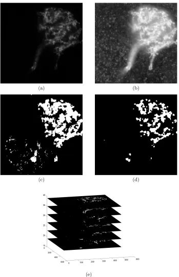
However, as shown in Fig.2(c), due to the existence of the background noise in the image stack (as shown in the ‘noise boosted’ image Fig.2(b), it is possible to get false alarms in the segmentation (Fig.2(c)) if only the wavelet likelihood is used. This occurs because some noise features may have wavelet features similar to the object regions. In this work, we introduce the global intensity likelihood as a means of discriminating against low intensity noise regions.

3.2 Global Intensity Likelihood

From Fig.2(a&b), we can see that the intensity of the background noise is close to the background brightness and is significantly different from the object brightness. Also, as shown in Fig.3, the ‘background’ intensity and the ‘object’ intensity are separable from each other in the histogram. Intuitively, the ‘object’ and ‘background’ intensity in the image can be fitted by two different Gaussian-pdfs. The parameters of the pdfs are estimated by fitting two Gaussian pdfs separately to the ‘object’ and ’background’ pixels collected from the segmented training images mentioned in Section 3.1.3. However, a pixel with higher intensity value is overwhelmingly likely to be the ‘object’, and conversely, a pixel is likely to be the ’background’ when the intensity is low. Since Gaussian pdf for the object will be small for high intensities, we instead use two Gaussian cumulative density functions (cdf) to estimate the ‘relative probabilities’ of a given pixel being ‘object’ or ’background’ as follows

pG(Is(x)|bs(x)) =







1−cdf(Is(x)|θG(β = 0))

(a) (b)

(c) (d)

(e)

Figure 3. Histogram of global intensity of the image stack. There are two peaks in the histogram where the peak with a mean at approximate 40belongs to ‘object’ and the other narrower peak belongs to ‘background’. We model both peaks with Gaussian-pdfs.

(6)

where θG(β) = {µG(β), σG2(β)} are the mean and the variance of the fitted Gaussain-pdf for ‘object’ or ’back-ground’ intensity. The result of the segmentation model with both the wavelet-likelihood and the global intensity likelihood is given in Fig.2(d), and obviously, the background noise features are removed while comparing to Fig.2(c) which is based on the wavelet-likelihood only.

The combination of the wavelet-likelihood and the global intensity likelihood forms the intra-slice likelihood in Eq.(4), and solves the irregular brightness problem while rejecting low intensity noise textures. The vertical likelihood in Eq.(4) that overcomes the out-of-focus problem is described in the following section.

3.3 Local Intensity Likelihood

The 2nd_{challenge of the synaptic object segmentation is the presence of out-of-focus features in the image stack.} The out-of-focus features are usually dimmer, thinner and more smooth than the in-focus features, however a synaptic object can have ‘branches’ with different thickness in the images and also, as discussed in Section 1, the fluorescent material is distributed unevenly over the synapse and hence appears with irregular brightness in the images. In other words, a relatively dimmer and thinner feature can be in-focus in the given image slice while a bright and thick feature is out-of-focus. Consequently, the determination of whether an object feature is in-focus or out-of-focus can not rely only on a single image slice, but instead, we should look through the image stack (as shown in Fig.4(a)) at the same local region of the object feature in the given image. Therefore, the determination is made based on local inter-slice information of the image stack rather than each individual horizontal planes. This key idea is injected to the Bayesian segmentation model as another likelihood term is capable of distinguishing the in-focus and out-of-focus features in a given image stack.

3.3.1 Vertical intensity profile

As shown in Fig.4, while considering the intensity distribution of a single point through the image stack vertically, the feature that is in-focus on a particular image slice corresponds to the highest value in the vertical intensity distribution (the ‘blue’ plot in Fig.4(b)), and the value decreases while the projection of the feature becomes more out-of-focus on the slices below or above the in-focus slice. Also, we assume that the value of the vertical intensity distribution will remain high while the feature is in-focus on multiple adjacent image slices. This happens when an object has a vertical orientation in the specimen. Consequently, the local intensity likelihoodpv of pixelxis estimated by a Gaussian pdf as following

pV(I1(x), Is(x), ..., IM(x)|bs(x)) =



 

 

1 , β= 0

exp[−(Is(x)−µv(x,s))2 2σ2

(a) (b)

Figure 4. Local vertical intensity profiles. (a) is the image stack in Fig.1 but highlighted by two vertical inter-slice lines at different pixel-wise locations. (b) shows the vertical intensity profiles corresponding to the locations labeled in (a)

(7)

where the meanµv(x, s) of the Gaussian-pdf is the maximum value of the local vertical intensity distribution of the same pixel sitexthrough the image slices. Since the intensity profile due to focus is assumed to be the same for all features in the same image stack, we use a fixed variance σ2

v = 2 for Gaussian-pdf. Note that the goal of the local intensity likelihood is to select the in-focus feature from the present of the out-of-focus version of the feature, hence this likelihood term is only applied to the ‘object’ probability and is ‘1’ for the ‘background’ probability.

In practice, when multiple features vertically coincide in an image stack, the vertical intensity profile of that local region would instead have multiple separate peaks in the intensity profile (’red’ plot in Fig.4(b)). In these cases, we fit different Gaussian-pdfs to each peak. We find the peaks using the intra-slice likelihood (the combined wavelet-likelihood and the global intensity likelihood) to give a rough segmentation of the image stack into dark or bright regions.

4. SMOOTHNESS FRAME PRIOR

So far, the likelihood terms have enabled the Bayesian model to overcome the irregular-brightness and out-of-focus problems. In fact, a single synapse is an object with connected ‘branches’ in the specimen, and therefore the ‘object’ features should also be connected as the ‘branches’ in the image stack. However, the likelihood terms described in the previous sections do not include any a priori knowledge of the smoothness properties of the object features in the image stack. For the cases that some synaptic ‘branches’ are stained with little fluorescent material in the specimen, the ‘weak’ appearance of those ‘branches’ in the image stack makes it likely to be classified as ‘background’ by the likelihood terms of the model. As a result, the object of a single synapse in the image stack may be ‘broken’ into several disconnected objects after segmentation.

In order to enhance the connection of such ‘weak’ branches, we inject a spatial smoothness prior to the segmentation model. This idea of this prior is to label a pixel as ‘object’ or background based on the label of the neighboring pixels. The smoothness is constrained by the ‘frame’ of the synaptic object, which can be considered as the skeleton of the connected ‘branches’ in the image stack.

4.1 Synaptic object frame

Figure 5. Illustrates the process of the Laplacian approach. The left column shows the image stack with different ‘reso-lutions’ by convolving with a 3D Gaussian kernelg3D. The stacks are arranged from fine to coarse. The middle column

contains the1st

order Laplacian features which obtained by abstracting the coarse image stack from the ’finer’ one ‘above’ it. The right column consists of the2nd_{Laplacian features that obtained by subtracting the1}st _{order Laplacian features at} different resolution levels.

stacks with finest features is placed on top of the pyramid and the coarsest version is located at the bottom. Here, a coarse image stack is generated by convolving the given image stack with a 3-D Gaussian like kernel, i.e. a ‘low-pass’ filter, and this coarse image stack is used to generate a coarser version at higher scale by convolving with the same ‘low-pass’ filter. A Laplacian approach is applied to the image pyramid to get the 1st _order Laplacian features by subtracting a coarse image stack from the adjacent finner image stack above it, and as a result, a pyramid of the 1st _{order Laplacian features at different scale is produced.}

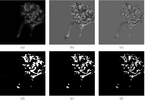
The frame of the synaptic object is then extracted from the Laplacian features by removing the negative values and filtering the positive values with the raw object mask (Fig.6(d)) mentioned in Section 3.3.1. A sample slice of the 1st _{order Laplacian features (Fig.6(b)) at scale 6 and the corresponding extracted object frame are} given in Fig.6(e), however this frame seems too coarse for the fine details of the synaptic object on the image. Therefore, in order to get ‘finer’ frame of the thin objects, we perform the Laplacian approach again but on the 1st _{order Laplacian features and do the abstraction on the resulted 2}nd _{order Laplacian features (Fig.6(c)). A} sample of the resulted finer frame for the corresponding thin synaptic branches is shown in Fig.6(f).

4.2 Frame prior

Since the ‘likely’ connections between the synaptic objects are now identified by the object frame, the a priori information of a given pixelxat image slicesderived from pixels in a 3D neighborhood N3D in the image stack

should be constrained by a binary object mask of the frame corresponding to the image stack, and hence the prior term is called ‘frame prior’.

(a) (b) (c)

(d) (e) (f)

Figure 6. Illustration of the Laplacian process by slice. (a) is an image slice of the original image stack in Fig.1. (b) is the1st

order Laplacian features of (a) at resolution ‘level 6’. (c) is the 2nd

order Laplacian features of (b). (d) is the initial segmentationb0

s for (c). (e) is the 1

st _{order object frame of (a) by thresholding the positive 1}st _{order Laplacian} features in (b) and filtered by (d). (f ) is the2nd

order object frame of (a) by thresholding the positive2nd

pS(bs(x)|b1(x), ..., bs−1(x), bs+1(x), ..., bM(x)) =                                    λ X y_i∈N3D

{ωi|1−BF(yi)||1−bs(yi)|} , BF(x) = 0 &β= 0

(1−λ) X

y_i∈N3D

{ωi|1−bs(yi)|} , BF(x) = 1 &β= 0

(1−λ) X

y_i∈N3D

{ωi|bs(yi)|} , BF(x) = 0 &β= 1

λ X y_i∈N3D

{ωi|BF(yi)||bs(yi)|} , BF(x) = 1 &β= 1

ωi=

|x−yi|

P

y_i∈N3D|x−yi|

(8)

where ωi is a set of normalized neighbor distances. Furthermore, the ‘strength’ of ‘frame constrained’ part is controlled by the ratioλ∈(0,1) in order to vary the ‘strength’ of the connections between the synapses.

5. OPTIMIZATION

The Bayesian framework using the proposed likelihoods and prior is optimized using the Iterated Conditional Modes (ICM) process.13 _{To initialize the optimization, an initial estimate of the segmentations for each slice,} bs, are evaluated using the Maximum Likelihood (ML) estimate. We then apply the ICM procedure to update

each slice segmentation,bs, in turn by finding theMaximum a Posteriori (MAP) estimate from Eq.(3). When

estimating the prior probability at each iteration, a fixed estimate of the synapse frameBF(x) calculated at the start of the process is used. We use a total of 5 iterations over the entire stack. From our experience, this allows for the segmentation to converge sufficiently. Furthermore, in our experiments, the weights{αW(·), αG(·), αV(·)} in Eq.(4) are set asαW(0) = 1.6,αW(1) = 1,αG(0) = 1,αG(1) = 2,{αV(0) = 1,αV(1) = 1 andλis set to 0.8.

6. RESULTS

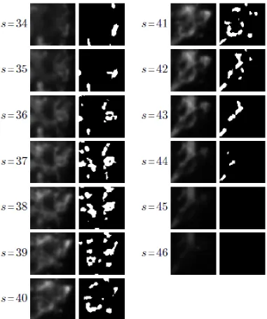
The 3D segmentation result of the a given sample image stack is given in Fig.1(b). As it is difficult to visualize a 3D segmentation, we have selected small samples of the image stack and illustrated the segmentations for a number of slices in the stack (Fig.7-Fig.10). Although this representation is not ideal for viewing the vertical relationships in the segmentation masks, it does allow us to demonstrate the effectiveness of aspects of our algorithm.

As shown in Fig.7 to Fig.10, our Bayesian mode has successfully segmented the in-focus synaptic features in both bright regions dim regions. For example, in Fig.7, the bright feature on the left of ‘slice 9’ is selected while the dimmer sharp in-focus features in ‘slice 15’ are also detected. The effectiveness of the vertical likelihood in detecting the in-focus regions can be seen in Fig.8. As shown in center of ‘slice 4’ to ‘slice 14’, when the object becomes brighter, there are more in-focus features being detected, but when it becomes dimmer in the later slices, there are less features being selected. However in some slices, like ‘slice 17’ in Fig.8 and ‘slice 44’ in Fig.9, the in-focus constraint is too strict so that the ‘relatively’ in-focus features are unselected. The reason of this ‘false negative’ is that we use a fixed variance σ2

v = 2 for the vertical inter-slice intensity profile. A potential approach to improve in-focus detection is using an adaptive variance. Furthermore, effectiveness of the frame prior is can seen in ‘slices 33 and 34’ in Fig.10, the in-focus features with ‘blob’ appearance would be detected as individual spots by only the likelihoods but are detected as elongated synaptic features.

7. CONCLUSION

In this paper, we introduce a Bayesian model for segmenting 3D synaptic objects from a given stack of specimen image slices captured using a fluorescent confocal microscope. The key intra-slice wavelet-likelihood provides a degree of luminance invariance in order to detect the synaptic features with irregular brightness. The other core likelihood based on the vertical inter-slice intensity profile enables the model to distinguish between in-focus and out-of-in-focus features. Furthermore, a novel frame prior is introduced to direct spatial smoothness along the skeleton of the synapses. Our model gives a plausible segmentation of synapses that requires manual segmentation in only one slice to train the Gaussian mixture models used for estimating the wavelet-likelihood. Further work on this problem will focus on using graph-cut optimization with our Bayesian framework. Using graph-cuts is advantageous as it finds the globally optimal labelling for a binary segmentation problem and hence is insensitive to any initialization.

REFERENCES

1. Barbee, S. A., Estes, P. S., Cziko, A.-M., Hillebrand, J., Luedeman, R. A., Coller, J. M., Johnson, N., Howlett, I. C., Geng, C., Ueda, R., Brand, A. H., Newbury, S. F., Wilhelm, J. E., Levine, R. B., Nakamura, A., Parker, R., and Ramaswami, M., “Staufen- and fmrp-containing neuronal rnps are structurally and functionally related to somatic p bodies,”Neuron52(6), 997–1009 (2006).

2. Bramham, C. R. and Wells, D. G., “Dendritic mrna: transport, translation and function,” Nature reviews. Neuroscience8(10), 776–789 (2007).

3. Hillebrand, J., Pan, K., Kokaram, A., Barbee, S., Parker, R., and Ramaswami, M., “The me31b dead-box helicase localizes to postsynaptic foci and regulates expression of a camkii reporter mrna in dendrites of drosophila olfactory projection neurons,”Frontiers in Neural Circuits 4, 121 (2010).

4. Pan, K., Hillebrand, J., Ramaswami, M., and Kokaram, A., “Gaussian mixture models for spots in mi-croscopy using a new split/merge em algorithm,” IEEE International Conference on Image Processing (ICIP’10) , 3645–3648 (2010).

5. Niemisto, A., Korpelainen, T., Saleem, R., Yli-Harja, O., Aitchison, J., and Shmulevich, I., “A k-means seg-mentation method for finding 2-d object areas based on 3-d image stacks obtained by confocal microscopy,” in [Engineering in Medicine and Biology Society, 2007. EMBS 2007. 29th Annual International Conference of the IEEE], 5559 –5562 (aug. 2007).

6. Long, F., Peng, H., and Myers, E., “Automatic segmentation of nuclei in 3d microscopy images of c.elegans,” in [Biomedical Imaging: From Nano to Macro, 2007. ISBI 2007. 4th IEEE International Symposium on], 536 –539 (april 2007).

7. Gouaillard, A., Mosaliganti, K., Gelas, A., Souhait, L., Obholzer, N., and Megason, S., “Streaming level set algorithm for 3d segmentation of confocal microscopy images,” in [Engineering in Medicine and Biology Society, 2009. EMBC 2009. Annual International Conference of the IEEE], 3621 –3624 (sept. 2009). 8. Garza-Jinich, M., Meer, P., and Medina, V., “Robust retrieval of three-dimensional structures from image

stacks,”Medical Image Analysis3(1), 21–35 (1999).

9. Ivan W. Selesnick, R. G. B. and Kingsbury, N. G., “The dual-tree complex wavelet transform,”IEEE Signal Processing Magazine 22(6), 123–151 (2005).

10. Comaniciu, D. and Meer, P., “Mean shift: A robust approach toward feature space analysis,”IEEE Trans. Pattern Anal. Mach. Intell.24, 603–619 (May 2002).

11. Burt, P. and Adelson, E., “The laplacian pyramid as a compact image code,” Communications, IEEE Transactions on31, 532 – 540 (apr 1983).

12. Hertzmann, A., “Painterly rendering with curved brush strokes of multiple sizes,” in [Proceedings of the 25th annual conference on Computer graphics and interactive techniques],SIGGRAPH ’98, 453–460, ACM, New York, NY, USA (1998).