Numerical simulation of EVA in thermal power plants based on system dynamics

Journal of Chemical and Pharmaceutical Research, 2014, 6(5):368-373

Research Article

_{CODEN(USA) : JCPRC5}

ISSN : 0975-7384

Numerical simulation of EVA in thermal power plants based on

system dynamics

Shuliang Liu

and Qianyun Liu

School of Economics and Management, North China Electric Power University, Baoding, Hebei, China

____________________________________________________________________________________________

ABSTRACT

Based on the theory of system dynamics, this paper preliminarily builds simple numerical simulation model of economic value added ( referred to as EVA) in thermal power plants. This model simulates EVA in thermal power enterprises after considering many factors. At the same time, it analyzes the main factors which affect EVA in order to provide some help for management in thermal power plants.

Key words: System dynamics; EVA; simulation model

____________________________________________________________________________________________

INTRODUCTION

Power generation industry is the backbone of our energy industry and it plays an important role in promoting the development of our national economy. The phenomenon of ignoring cost of equity capital in power generation plants is serious on basis of which State-owned Assets Supervision and Administration Commission (SASAC) began to exert EVA in the performance appraisal system in 2005 and they made an all-round implementation in 2010. SASAC then issued Guidance on Strengthening Value Administration Based on the Core of EVA in Central Enterprises in 2014. Therefore, the philosophy of EVA value management is becoming prevalent among central enterprises including thermal power plants.

EVA was put forward by Stern Steward company in 1991 and it compensates the lack of distinction between the cost of debt capital and equity capital [10]. At present, the domestic research about EVA primarily concentrates on the following two aspects: Firstly, people introduce the theory of EVA. Shengli Du discussed the concept, calculation and adjustments related to accounting reports when EVA was applied [1]. As a tool of management control, EVA descends from residual income and has been applied in many fields, such as setting target, performance appraisal, and so on [7]. Secondly, people have done much empirical research containing correlative analysis of relationship between EVA, incentive systems and enterprise value, together with the compare between EVA and traditional performance appraisal indexes. This gives further evidence that EVA will play an important role in promoting enterprises’value [8]. However, the research on integration of EVA and the theory of system dynamics is relatively little.

This text preliminarily builds the numerical simulation of EVA in a thermal power plant based on system dynamics. This simulation is composed of many parts, such as state variables, rate variables, auxiliary variables, constants and so on and I try my best to take factors influencing EVA into consideration as much as possible. This model can help marketing managers intuitively see the feedback relationship between variables so as to make better decisions.

THE THEORETICAL ANALYSIS OF SYSTEM DYNAMICS MODEL

and features of the system, which leads to the main simulation of structures and functions. The role of optimization in SD studies is not to replace experience-based knowledge, but instead to viewpoints, facilitates, and expand the heuristic exploration of a model [6].At the same time, combining with computer technology is an important means of modeling[5] and computer-aided modeling[4] arose accompanied by the the appearance of SD.Currently, SD has gained extensive application in many fields and shows great advantages especially in dealing with those complex system problems, which have characteristics of nonlinear, feedback and dynamics [3]. EVA simulation model for thermal power plants is suitable for SD to study because of its dynamics and complexity of its structure. SD is basically modeled according to the conceptual model, the structural model and the simulation model, namely causal loop diagram, flow diagram and simulation carried out [9] and this paper builds EVA model in this order.

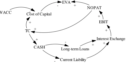
Feedback is really very important in SD. Many structures of complicated systems are described by causal loop diagrams which are powerful tools and the basis of system dynamics. With the software of Vensim PLE, this paper discusses the causal loop diagrams of numerical simulation of EVA, as is shown in Figure 1.

WACC _{Cost of Capital}

TC

EVA

CASH _{Long-term Loans}

Current Liability

Interest Exchange EBIT

NOPAT +

+

+

-+ +

+ + +

-+

Fig. 1: The causal loop diagram of EVA simulation

Causal loop diagram is mainly composed of the following three parts: causality, causal key and feedback loop [2]. With the overall understanding of the system, causality is the foundation for modeling. Feedback is the core of SD and the complex systems in SD are expressed by causal loop diagrams. Causal loop diagram is formed by two or more causal keys end to end.

As is shown in Figure 1, the causal relationship between TC and cost of capital is connected by lines with arrows. And the positive sign besides the arrow which is called positive causal chain together with the line and the arrow indicates positive causal relationship, and vice versa [2]. At the same time, there is a negative feedback loop in Figure 1. It illustrates that if the amount of TC increases, the cash in enterprises will then increase and liabilities will fall, interest expenses will decrease, EBIT will decline, NOPAT will drop. At the end, TC will come down.

Flow diagram is an important component of SD. On the basis of causal loop diagram, it carries more important information and aids in a fuller and deeper understanding of the structure of SD. The diagram is composed of many parts, such as state variables, rate variables shown in Figure 2 [2], auxiliary variables, constants and so on.

State Variable

Rate Variable b _{Rate Variable a}

Fig. 2 Flow diagram of system dynamics

The diagram is essentially first-order differential equation with the character of nonlinear autonomous delay. But some information is expressed by table functions, time functions and other functions.

THE COMPOSITION OF EVA SIMULATION MODEL

Suppose the interrelated social environment and laws and regulations remain constant and the plant operations sound. The sales of heat and miscellaneous gains are neglected during the process of constructing this model on account of the main sales of electricity. In addition, this model consists of multiple auxiliary variables and constants, for example per-unit cost and revenue of power sales which are considered to be constants.

Some parts of the variable equations in this model are shown as follows:

Table 1: Meaning of the variables in the system flow chart

Variable Name Formula Unit

EVA NOPAT-Cost of Capital Ten Thousand Yuan

Cost of Capital TC*WACC Ten Thousand Yuan

TC Debt Capital + Equity Capital -Construction in Process Ten Thousand Yuan Debt Capital Current Liability + Long-term Loans + Long-term Liabilities due within one year Ten Thousand Yuan Equity Capital Capital Stock + Minority Interest + Investment Capital Adjustment Ten Thousand Yuan Investment Capital Adjustment Depreciation Reserves + Credit Balance of Deferred Tax Ten Thousand Yuan WACC Cost of Debt after Tax*(Debt Capital/Total Capital)+Cost of Equity*(Equity

Capital/Total Capital)

NOPAT EBIAT + Minority Interest Income + Depreciation Reserves-Debit Balance of

Deferred Tax Ten Thousand Yuan

EBIAT EBIT*(1-Rate of Income Tax) Ten Thousand Yuan

EBIT Net Profit + Interest + Income Tax Ten Thousand Yuan

Gross Operating Profit Revenue from Electricity Sales-Operating Expenses-Cost of Electricity Sales

-Administrative Expenses-Finance Charges-Sales Tax and Extra Charges Ten Thousand Yuan

Depreciation Reserves in this model includes Fixed Assets Depreciation Reserves, Long-term Investments Depreciation Reserves, Inventory Falling Price Reserves and something else. Of course, we can adjust correlative variables accordingly.

The constants are as follows: the rate of Current Liability is 0.05022 and the rate of Long-term Loans is 0.06156. Some other variables, such as Current Liability, Long-term Loans and Expenses, are illustrated by time functions presenting the changing relationship between variables and time. Take Current Liability for example: Current Liability=WITH LOOKUP(Time,

([(2007,0)-(2001,4000)],(2007,21236),(2008,21236),(2009,21236),(2010,21236),(2011,11236))).

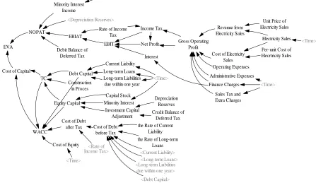
The construction of EVA simulation model is shown as follows:

EVA

NOPAT

Minority Interest Income

EBIAT

Debit Balance of Deferred Tax

Rate of Income Tax EBIT Income Tax Net Profit Interest Gross Operating Profit Revenue from Electricity Sales

Cost of Electricity Sales Operating Expenses Administrative Expenses Finance Charges

Sales Tax and Extra Charges

Unit Price of Electricity Sales

Electricity Sales Per-unit Cost of Elecrtricity Sales

Cost of Capital TC WACC Debt Capital Construction in Proces Equity Capital Current Liability Long-term Loans Long-term Liabilities

due within one year Capital Stock Minority Interest Investment Capital Adjustment Depreciation Reserves Credit Balance of

Deferred Tax Cost of Debt

after Tax Cost of Debt before Tax

the Rate of Current Liability the Rate of Long-term

Loans Cost of Equity

<Depreciation Reserves> <Time> <Time> <Time> <Time> <Time> <Current Liability> <Long-term Loans> <Long-term Liabilities

due within one year> <Debt Capital> <Rate of

RESULTS OF EVA SIMULATION

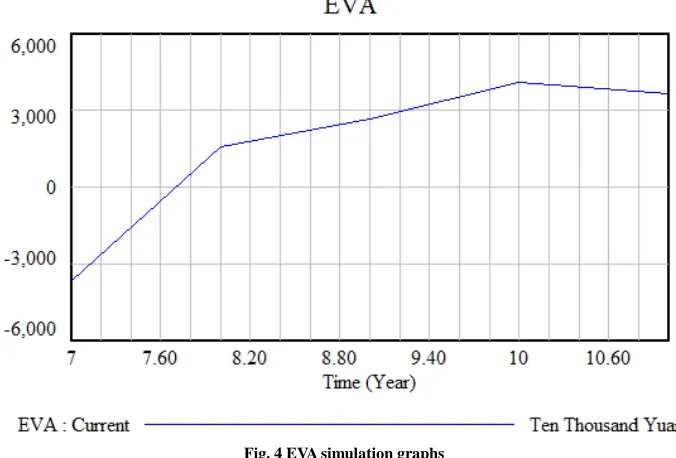
Combined with software of Vensim PLE, the numerical simulation of EVA in thermal plant based on system dynamics is as follows:

Fig. 4 EVA simulation graphs

The error analysis of EVA is shown in Table 2 and Figure 5 by means of comparing the actual value and the predicted value.

Table 2: Error analysis between actual value and predictive value of EVA

EVA (Year) 2007 2008 2009 2010 2011 Actual Value -3948.21 1575.93 2739.25 3806.13 3742.61 Predictive Value -3663.78 1565.71 2680.3 4080.71 3655.88 Relative Error -0.07204 -0.00649 -0.02152 0.072142 -0.02317

R e l a t i v e E r r o r

- 0 . 0 8 - 0 . 0 6 - 0 . 0 4 - 0 . 0 2 0 0 . 0 2 0 . 0 4 0 . 0 6 0 . 0 8

2 0 0 7 2 0 0 8 2 0 0 9 2 0 1 0 2 0 1 1

Y e a r

R e l a t i v e E r r o r

Fig. 5 Relative error graphs

From Table 2 and Figure 5 presented above, it is apparent that the relative tolerance between predicted value and actual value has a margin of error of plus or minus 8 percentage points on basis of which we conclude that the predictions are coincided with reality and this simulation model is relatively accurate.

ANALYSIS OF THE RESUILTS IN THIS MODEL

(1) Causes-tree is a structure chart reflecting causality. As is shown in Figure 6, the immediate cause of EVA is Cost of Capital and NOPAT which is conversely led to by TC, WACC and Debit Balance of Deferred Tax, Depreciation Reserves, EBIAT, Minority Interest Income respectively. This is just an cursory analysis.

Fig. 6 Causes-tree of EVA

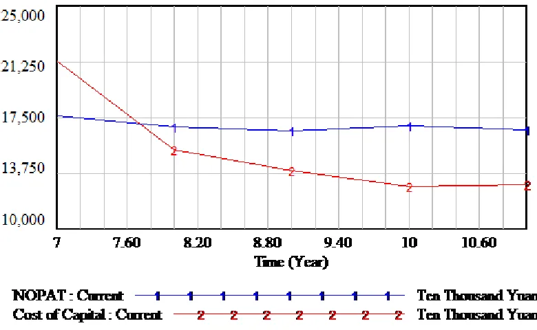
(2) Superficially, Cost of Capital and NOPAT are on the decrease whereas EVA is in the opposite case. In fact, the distance between Cost of Capital and NOPAT which have experienced an upturn shown in Figure 7 represents EVA. This proves the correctness of EVA simulation model.

Fig. 7 NOPAT and Cost of Capital simulation graphs

(3)As is shown in Table 3, neither unit price of electricity sales growth of 10 percent nor unit cost of electricity fall of 10 percent makes EVA fires on all cylinders on the ground of which we can make a further conclusion that both of this two factors have important influences on EVA.

Each generation plant faces great challenges and competition accompanied by the partition of power plants and power network and they need to devote themselves to raising generating capacity and reducing costs. The government exerts much impact on the price of sales and the thermal power plant should concentrate on costs of sales to achieve the best.

coordinating costs of coal-fired will plays a significant role in reducing costs. On the other hand, we can’t neglect other factors such as costs of fuel and coal incidentals and so on.

Table 3: Sensitivity analysis of EVA

Predicted Value of EVA (Ten Thousand Yuan)

Sensitivity Analysis of EVA (Ten Thousand Yuan) Year Original Simulated

Data

Unit Price Increased by 10%

Unit Cost Decreased by 10%

Unit Price Increased by 10%

Unit Cost Decreased by 10%

2007 -3663.78 3760.95 1488.1 -2.02652 -1.40617

2008 1565.71 8787.99 6577.13 4.612783 3.200733

2009 2680.3 9902.58 7691.72 2.694579 1.869724

2010 4080.71 11464.2 9203.95 1.809364 1.255478

2011 3655.88 11019.4 8765.32 2.014158 1.397595

CONCLUSION

The numerical simulation of EVA in this article analyses the structure and function of this model based on SD and the result is in well agreement with physical truth, which illustrates the correctness of this model. On the other hand, we find that determining the variables included in the model as comprehensively and accurately as possible and optimizing the sensitivity factors are very important for modeling. Af course, there is more work to be done for me to improve this model because of the limitation of my knowledge and this is where I need to do more .

Acknowledgments

The authors wish to thank the support of school of economics and management of North China Electric Power University in hebei, China and the help of my workmates , under which the present work was possible.

REFERENCES

[1] S. L. Du. Performance Evaluation of Enterprises’ Operating, Economic Science Publishing House, 1999. [2] Y. L. Xie, H. P. Yuan. System Dynamics in Financial Management Application, Metallurgical Industry Publishing House, 2008.

[3] Y. G Zhong, X. J. Jia. System Dynamics, Science Publishing House, 2012.

[4] H. C. Zhao. The Realization of Computer-aided Flow Diagram of SD, Systems Engineering, n.1, pp.39-42, 1990. [5] J. R. Burns et al. An Algorithm for Converting Signed Digraphsto Forrester Schematics, IEEE Tran,Syst.Man. Cybern.V.9, n.3, pp.115-124, 1979.

[6] R. Bailey, B. Bras, J. K. Allen. Using Response Surface to Improve the Search for Satisfactory Behavior in System Dynamics Models, System Dynamics Review, n.16, pp.75-90, 2000.

[7] Gao Chen, L. G. Tang. Integrated Mode of Management Control Tools: Theoretical Analysis and Innovation about Chinese Companies-Based on Research of Multiple Cases in Chinese State-owned Enterprises, Accounting Research, n.8, pp.68-75, 2007.

[8] G. H. Chi, Wang Zhi. Does EVA Promote Enterprises’ Value?-Based on Empirical Evidence of Chinese State-owned Quoted Enterprises, Accounting Research, n.11, pp.60-66, 2013.

[9] J. W. Forrester. Principles of Systems Cambridge, MA: Wright-Allen Press. 1968.