Numerical investigation of turning diffuser performance: validation and verification model II

14 -16 May 2015, Seri Iskandar, Perak

Numerical Investigation of Turning Diffuser

Performance: Validation and Verification-Model II

Normayati Nordin

Faculty of Mechanical and Manufacturing Engineering Universiti Tun Hussein Onn Malaysia

Batu Pahat, Malaysia [email protected]

Zainal Ambri Abdul Karim

Department of Mechanical Engineering Universiti Teknologi Petronas

Tronoh, Malaysia [email protected]

Safiah Othman

Faculty of Mechanical and Manufacturing Engineering Universiti Tun Hussein Onn Malaysia

Batu Pahat, Malaysia [email protected]

Vijay R. Raghavan

OYL Research & Development Centre OYL Research & Development Sdn Bhd

Sungai Buloh, Malaysia [email protected]

Abstract— This paper aims to validate the numerical

method used to intensively study the performance of turning diffuser. A 3-D turning diffuser of area ratio (AR=2.16), outlet inlet configurations (W2/W1=1.50, X2/X1=1.44) and inner wall

length (Lin/W1=3.99) operated at inflow Reynolds numbers, Rein

= 5.786 x 104- 1.775 x 105 was considered. Grid with appropriate size, y+ was occupied relatively in dense close to the walls. The quality and independency of grid was examined. The applicability of k- turbulence models, i.e. standard k- (ske), renormalization group k- (rngke) and realizable k- (rke) by means of adopting different near wall treatments to simulate the actual cases, was assessed. The enhanced wall treatment, y+1.2-1.7 adopted ske appeared as the best validated model, producing minimal deviation with comparable flow structures to the actual cases.

Keywords— CFD; turning diffuser; validation

INTRODUCTION

Diffusers are classified by their geometry. A diffuser that is introduced with no turn is known as a straight diffuser [1-3], whereas a diffuser introduced with certain angle of turn is called a turning diffuser or a curved diffuser [3-6]. Study of the geometry effect on diffuser performance has been of fundamental interest to researchers in the area of fluid mechanics since decades and it continues to grow [1-17].

The primary index used to measure the performance of a diffuser is outlet pressure recovery coefficient (Cp):

2 ) (

2

in in out p

V P P C

 

 (1)

where,

Pout= outlet static pressure (Pa)

Pin= inlet static pressure (Pa)  = flow density (kg/m3)

Vin= inlet air velocity (m/s)

The value of Cp indicates how much kinetic energy is

successfully converted to pressure energy. The main problem in achieving a high pressure recovery is flow separation, which results in non-uniform flow distribution and excessive energy losses. It is even worse, particularly when a 90o turn together with a diffusing effect is applied. The flow through a turning diffuser with 90o angle of turn is rather complex, apparently due to the expansion and sharp inflexion introduced along the direction of flow, causing strong adverse pressure gradient-driven streamwise vortices.

Computational fluid dynamics (CFD) as a tool has been widely employed by scientists and engineers in flow studies. The total dependence on experimental methods can be reduced by implementing the CFD techniques. There is basically a challenge in assigning the best model to represent the actual case when a complex flow is involved. The k- turbulence is the model introduced by Jones and Launder [7], which has been used widely in industry. This model along with appropriate setting of grid and wall boundary conditions managed to predict the onset flow separation accurately [2, 8]. There are several successful studies predicting the flow within a diffuser, which essentially employed k- turbulence model [2, 8-14].

14 -16 May 2015, Seri Iskandar, Perak

flows (Re<106) or flows with complex near wall phenomenon [16]. It requires very fine near-wall mesh, i.e.

y+1.0 capable of resolving the viscous sublayer to at least 10 cells within the inner layer.

In the present work, the applicability of k- turbulence models namely standard k- (ske), renormalization group

k- (rngke) and realizable k- (rke) by means of adopting standard wall functions, non-equilibrium wall functions and enhanced wall treatment to simulate the flow within a turning diffuser are assessed. A 3-D turning diffuser of area ratio (AR=2.16), outlet inlet configurations (W2/W1=1.50,

X2/X1=1.44) and inner wall length (Lin/W1=3.99) operated at

inflow Reynolds numbers, Rein= 5.786 x 104- 1.775 x 105 is

considered.

I. GEOMETRICAL DOMAIN AND BOUNDARY CONDITIONS

ANSYS DesignModeler was used to create the geometrical domain. As shown in Fig. 1, the inner-wall and center curves were constructed using quarter circles of radii

rin=12 cm and rm=15.6 cm respectively. The outer-wall

curve was shaped using circular-arcs tangent to the sequence of circles, thus an even area propagation between the inner and outer wall passages could be established relative to the center.

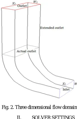
A three-dimensional flow domain in Fig. 2 was created by extruding the base object, i.e. solid line in Fig. 1 within angle of diffusion, =15.154o. The actual outlet was extended by a length equal to the center curve length, Lm to

remedy the flow, after which the pressure could be considered as the atmospheric pressure.

Three types of boundary conditions were imposed. At the solid wall, the velocity was zero due to the no-slip condition. The inlet velocity, Vin = 12.92 - 39.66 m/s was

varied respective to the Rein. At the outlet boundary, the

pressure was specified at the atmospheric pressure (0 gage pressure).

Fig. 1. Construction lines, i.e. dashed line of a 90o _{turning diffuser}

Fig. 2. Three dimensional flow domain

II. SOLVER SETTINGS

ANSYS Fluent 14.5 was used as a platform for the analysis. The flow was assumed to be incompressible, three-dimensional (x, y and z direction), fully-developed, steady state and isothermal. The gravitational effect was negligible. The Reynolds Average Navier Stokes (RANS) equations as follows were solved.

Continuity equation: 0    z w y v x u     

 ₍₂₎

x- momentum equation:

Mx S z w u y v u x u z u y u x u x P z u w y u v x u

u           

                     

 ( 2) ( ) ( )

2 2 2 2 2 2 (3) y- momentum equation:

My S z w v y v x v u z v y v x v y P z v w y v v x v

u           

                     

 ( ) ( 2) ( )

2 2 2 2 2 2 (4) z- momentum equation:

Mz S z w y w v x w u z w y w x w z P z w w y w v x w

u           

                     

 ( ) ( ) ( 2)

2 2

2 2

2

2 ₍₅₎

14 -16 May 2015, Seri Iskandar, Perak III. GRID INDEPENDENCE STUDY

The grid was generated using ANSYS ICEM CFD with the size of wall-adjacent cell, y+ was prescribed as follows:

v u y y  

(6) where,

y = normal distance from the wall (m) u= friction velocity (m/s)

= kinematic viscosity (m3/s)

The friction velocity was estimated as:

2 f

w _V C

u  

 



(7)

where,

V= flow velocity (m/s)

4 / 1

Re 039 . 0 2

 

f

C

(8)

It is important to cautiously refine the grid close to the wall because this region involves significant change of variables. Hexahedral mesh has been verified previously to provide the best continuity and fitted the curved geometries well [10, 11]. However, it was beyond the capacity of the computer in this study to generate uniform hexahedral mesh with adequate refinement to represent the actual flow. The adequate refinement particularly near to the wall was achieved merely by applying hybrid grid, i.e. tetrahedral and wedge elements.

As presented in Table 1, for standard and non-equilibrium wall functions y+63 was applied. Whereas, y+1.2-1.7 was set for enhanced wall treatment. Fig. 3 shows that the grid was uniformly scattered throughout the diffuser with the skewness of elements for all cases less than 0.3.

Table 1. Size of grid

Fig. 3. Hybrid grid

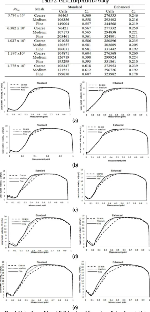
The grid independency was checked as depicted in Table 2. The ske turbulence model was applied for three kinds of grids, i.e. coarse, medium and fine by means of adopting standard and enhanced near wall treatments. The medium mesh was chosen as final meshing since it provided relatively small change of Cp to the fine mesh with

reasonable CPU time. Fig. 4 shows the effect of refining the grid on the outlet velocity profile extracted across the center of actual outlet. Basically, there was insignificant change of velocity profiles particularly between the medium and fine mesh.

Table 2. Grid independence study

(a)

(b)

(c)

(d)

(e)

Fig. 4. Velocity profiles of 3-D turning diffuser by refining the grid (a) Rein=5.786 x 104, (b) Rein=6.382 x 104, (c) Rein=1.027 x 105, (d)

14 -16 May 2015, Seri Iskandar, Perak

IV. VALIDATION OF NUMERICAL METHOD

Validation of numerical work was carried out by comparing the simulation results with the experimental results [17]. The parameters considered for validation purpose are velocity profile across the center of actual outlet, Vi and outlet pressure recovery coefficient, Cp.

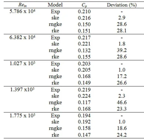
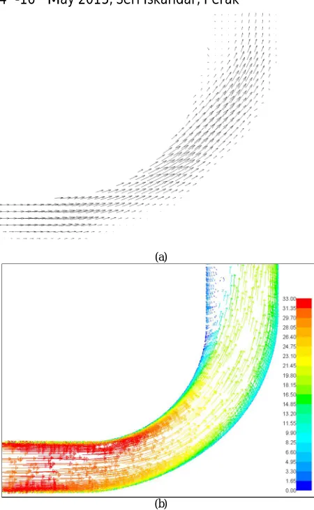
As is seen in Fig. 5, velocity profiles modelled by CFD satisfy the experiment optimally in all cases when enhanced near wall treatment is adopted. Table 3 shows that the ske model adopted enhanced near wall treatment consistently gives less than 5% of numerical deviation. As is shown in Table 4, the least deviation of Cp, 1.0-2.9% and comparable

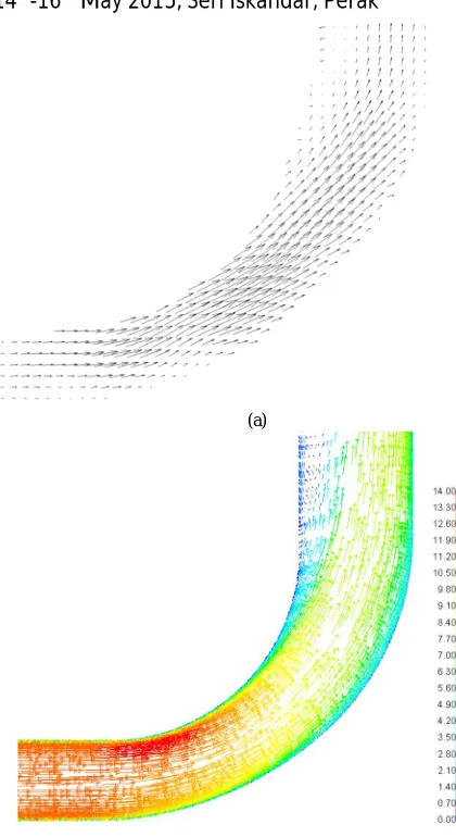
flow structures with almost similar onset flow separation between numerical and experimental are obtained when ske+enhanced wall treatment model is applied (see Fig. 6-10).

(a)

(b)

(c)

(d)

(e)

Fig. 5: Outlet velocity profiles of 3-D turning diffuser (a) Rein=5.786 x 104_{, (b) Rein=6.382 x 10}4_{, (c) Rein=1.027 x 10}5_{, (d) Rein=1.397 x10}5 _and

(e) Rein=1.775 x 105

Table 3: Average deviation of velocity distribution by applying ske model adopted different near wall treatment

Table 4: Deviation of Cp by applying different CFD model adopted

14 -16 May 2015, Seri Iskandar, Perak

(a)

(b)

Fig. 6. Flow structure within the turning diffuser operated at Rein=5.786 x 104 (a) experimental and (b) ske + enhanced wall treatment

(a)

(b)

Fig. 7. Flow structure within the turning diffuser operated at Rein=6.382 x 104 (a) experimental and (b) ske + enhanced wall treatment

(a)

(b)

14 -16 May 2015, Seri Iskandar, Perak

(a)

(b)

Fig. 9. Flow structure within the turning diffuser operated at Rein=1.397 x 105 (a) experimental and (b) ske + enhanced wall treatment

(a)

(b)

Fig. 10. Flow structure within the turning diffuser operated at Rein=1.775 x 105 (a) experimental and (b) ske + enhanced wall treatment

V. CONCLUSION

In conclusion, the current work validates the numerical method used to intensively study the performance of turning diffusers. The ske adopted enhanced wall treatment, y+ 1.2-1.7 appeared as the best model to represent the actual cases.

REFERENCES

[1] G. Gan and S.B. Riffat, “Measurement and computational fluid dynamics prediction of diffuser pressure-loss coefficient,” Applied Energy, vol. 54(2), pp. 181-195, 1996. [2] W.A. El-Askary and M. Nasr, “Performance of a bend diffuser system: Experimental and

numerical studies,” Computer & Fluids, vol. 38, pp.160-170, 2009.

[3] R.K. Sullerey, B. Chandra, and V. Muralidhar, "Performance comparison of straight and curved diffusers," J. of Def. Sci., vol. 33, pp. 195-203, 1983.

[4] N. Nordin, V.R. Raghavan, S. Othman and Z.A.A. Karim,“Compatibility of 3-Dturning diffusers by means of varying area ratios and outlet-inlet configurations", ARPN Journal of Engineering and Applied Sciences, Vol. 7, No. 6, pp 708-713, 2012. [5] T.P. Chong, P.F. Joseph and P.O.A.L. Davies, “A parametric study of passive flow

control for a short, high area ratio 90 deg curved diffuser,” J. Fluids Eng., vol. 130, 2008.

[6] C.J. Sagi and J.P. Johnson, “The design and performance of two-dimensional, Curved Diffusers,” J. Basic Eng. ASME, vol. 89, pp. 715-731, 1967.

[7] W.P. Jones, B.E., Launder, “The calculation of low-reynolds number phenomena with a two equation model of turbulence,” Int. J. Heat Mass Transfer, vol. 6, pp. 1119-1130, 1973.

[8] D. Xu, M. A. Leschziner, B. C. Khoo, and C. Shu, "Numerical prediction of separation and reattachment of turbulent flow in axisymmetric diffuser," Computers & Fluids, vol. 26, pp. 417-423, 1997.

[9] Y.T. Yang and C. F. Hou, "Numerical calculation of turbulent flow in symmetric two-dimensional diffusers," Acta Mechanica, vol. 137, pp. 43-54, 1999.

[10] M.K. Gopaliya, M. Kumar, S. Kumar, and S. M. Gopaliya, "Analysis of performance characteristics of S-shaped diffuser with offset," Aerospace Science & Tech., vol. 11, pp. 130-135, 2007.

[11] M. K. Gopaliya, P. Goel, S. Prashar, and A. Dutt, "CFD Analysis of performance characteristics of S-shaped diffusers with combined horizontal and vertical offsets,"

Computer & fluids, vol. 40, pp. 280-290, 2011.

[12] I.H. Ibrahim, E.Y.K. Ng, K. Wong, and R. Gunasekaran, "Effects of centerline curvature and cross-sectional shape transitioning in the subsonic diffuser of the f-5 fighter jet," J. Mechanical and Science Technology, vol. 22, pp. 1993-1997, 2008.

[13] S. Jakirlic, G. Kadavelil, M. Kornhaas, M. Schäfer, D.C. Sternel, and C. Tropea, "Numerical and physical aspects in LES and hybrid LES/RANS of turbulent flow separation in a 3-D diffuser," International Journal of Heat and Fluid Flow, vol. 31, pp. 820-832, 2010.

[14] N. Nordin, V. R. Raghavan, S. Othman and Z. A. A. Karim, “Numerical investigation of turning diffuser performance by varying geometric and operating parameters”,

Applied Mechanics and Materials Journal, Vol. 229-231, pp. 2086-2093, 2012. [15] B. E. Launder and D. B. Spalding, "The numerical computation of turbulent flows".

Computer Methods in Applied Mechanics and Engineering, vol. 3, pp. 269–289, 1974. [16] ANSYS FLUENT User’s Guide, release 14.0, Canonsburg, USA, 2011.