Performance Trajectories and Performance Gaps as Achievement Effect-Size Benchmarks for Educational Interventions

(1)

MDRC Working Papers on Research Methodology

Performance Trajectories and Performance Gaps

as Achievement Effect-Size Benchmarks

for Educational Interventions

Howard S. Bloom MDRC Carolyn J. Hill

Georgetown Public Policy Institute Alison Rebeck Black

MDRC Mark W. Lipsey

Vanderbilt Institute for Public Policy Studies

(2)

(3)

Acknowledgments

The research on which this article is based received support from the Institute of Education Sciences in the U.S. Department of Education, the Judith Gueron Fund at MDRC, and the Wil-liam T. Grant Foundation. The authors thank Larry Hedges for his helpful input.

The findings and conclusions in this report do not necessarily represent the official positions or policies of the funders.

Dissemination of MDRC publications is supported by the following funders that help finance MDRC’s public policy outreach and expanding efforts to communicate the results and implica-tions of our work to policymakers, practitioners, and others: The Ambrose Monell Foundation, Bristol-Myers Squibb Foundation, The Kresge Foundation, and The Starr Foundation. MDRC’s dissemination of its education-related work is supported by the Bill & Melinda Gates Foundation, Carnegie Corporation of New York, and Citi Foundation. In addition, earnings from the MDRC Endowment help sustain our dissemination efforts. Contributors to the MDRC Endowment in-clude Alcoa Foundation, The Ambrose Monell Foundation, Anheuser-Busch Foundation, Bristol-Myers Squibb Foundation, Charles Stewart Mott Foundation, Ford Foundation, The George Gund Foundation, The Grable Foundation, The Lizabeth and Frank Newman Charitable Foundation, The New York Times Company Foundation, Jan Nicholson, Paul H. O’Neill Charitable Founda-tion, John S. Reed, The Sandler Family Supporting FoundaFounda-tion, and The Stupski Family Fund, as well as other individual contributors.

For information about MDRC and copies of our publications, see our Web site: www.mdrc.org.

(4)

(5)

Abstract

This paper explores two complementary approaches to developing empirical benchmarks for achievement effect sizes in educational interventions. The first approach characterizes the natural developmental progress in achievement by students from one year to the next as effect sizes. Data for seven nationally standardized achievement tests show large annual gains in the early elementary grades, followed by gradually declining gains in later grades. A given intervention effect will therefore look quite different when compared with the annual progress for different grade levels. The second approach explores achieve-ment gaps for policy-relevant subgroups of students or schools. Data from national and dis-trict-level achievement tests show that, when represented as effect sizes, student gaps are relatively small for gender and much larger for economic disadvantage and race/ethnicity. For schools, the differences between weak schools and average schools are surprisingly modest when expressed as student-level effect sizes. A given intervention effect viewed in terms of its potential for closing one of these performance gaps will therefore look very dif-ferent, depending on which gap is considered.

(6)

(7)

List of Tables, Figures, and Boxes

Table

1 Annual Reading Gain in Effect Size from Seven Nationally Normed

Tests 10 2 Annual Reading Gain in Effect Size from School District Data:

Com-parison of Cross-Sectional and Longitudinal Gaps in Two Distracts 14 3 Average Annual Gains in Effect Size for Four Subjects from

National-ly Normed Tests 16

4 Demographic Performance Gap in Mean NAEP Scores, by Grade (in

Effect Size) 21

5 Demographic Performance Gap in SAT 9 Scores from a Selected

School District, by Grade (in Effect Size) 23

6 Performance Gap in Effect Size Between “Average” and “Weak”

Schools (50th_{and 10}th_percentiles) ₂₈

A.1 Reading: Standard Deviations of Scaled Scores by Grade for Each

Test 35

C.1 Annual Math Gain in Effect Size from Six Nationally Normed Tests 46

C.2 Annual Science Gain in Effect Size from Six Nationally Normed Tests 47

C.3 Annual Social Studies Gain in Effect Size from Six Nationally

Normed Tests 48

Figure

1 Mean Annual Reading Gain in Effect Size 12

2 Illustration of Variation in Mean Annual Reading Gain 18

3 “Weak” and “Average” Schools in a Local School Performance

(10)

(11)

Introduction

In educational research, the effect of an intervention on academic achievement is of-ten expressed as an effect size. The most common effect size metric for this purpose is the

standardized mean difference,1_{which is defined as the difference between the mean}

out-come for the intervention group and that for the control or comparison group, divided by the common within-group standard deviation of that outcome. This effect size metric is a statis-tic and, as such, represents the magnitude of an intervention in statisstatis-tical terms, specifically in terms of the number of standard deviation units by which the intervention group outper-forms the control group. That statistical magnitude, however, has no inherent meaning for the practical or substantive magnitude of the intervention effect in the context of its applica-tion. How many standard deviations of difference represent an improvement in achievement that matters to the students, parents, teachers, administrators, or policymakers who may question the value of that intervention?

Assessing the practical or substantive magnitude of an effect size is central to three stages of educational research. It arises first when the research is being designed, and sions must be made about how much statistical precision or power is needed. Such deci-sions are framed in terms of the minimum effect size that the study should be able to detect with a given level of confidence. The smaller the desired “minimum detectable effect,” the larger the study sample must be. But how should one choose and justify a minimum effect size estimate for this purpose? The answer to this question usually revolves around consid-eration of what effect size would represent a practical effect of sufficient importance in the intervention context, such that it would be negligent if the research failed to identify it at a statistically significant level.

The issue of interpretation arises next toward the end of a study, when researchers are trying to decide whether the intervention effects they are reporting are large enough to be substantively important or policy-relevant. Here also, the simple statistical representation of the number of standard deviation units of improvement produced by the intervention begs the question of what it means in practical terms. This issue of interpretation arises yet again when researchers attempt to synthesize estimates of intervention effects from a series of studies in a meta-analysis. The mean effect size across studies of an intervention that summarizes the overall findings is also only a statistical representation that must be inter-preted in practical or substantive terms for its importance to be properly understood.

1_{For discussions of alternative effect size metrics see: Cohen (1988); Glass, McGaw, and Smith}

(1981); Grissom and Kim (2005); Fleiss (1994); Hedges and Olkin (1985); Lipsey and Wilson (2001); Rosenthal (1991); Rosenthal (1994); and Rosenthal, Rosnow, and Rubin (2000).

(12)

2

To interpret the practical or substantive magnitude of effect sizes, it is necessary to invoke some appropriate frame of reference external to their statistical representation that can, nonetheless, be connected to that statistical representation. There is no inherent prac-tical or substantive meaning to standard deviation units. To interpret them we must have benchmarks that mark off magnitudes of recognized practical or substantive significance in standard deviation units. We can then assess an intervention effect size with those bench-marks. There are many substantive frames of reference that can provide benchmarks that might be used for this purpose, however, and no one benchmark will be best for every in-tervention circumstance.

This paper develops and explores two types of empirical benchmarks that have broad applicability for interpreting intervention effect sizes for standardized achievement tests in educational research. One benchmark considers those effect sizes relative to the normal achievement gains children make from one year to the next. The other considers them in relation to policy-relevant achievement gaps between subgroups of students and schools achieving below normative levels and those whose achievement represents those normative levels. Before discussing these benchmarks, however, we must first consider several related issues that provide important contextual background for that discussion.

Effect Size Variants, Statistical Significance, and Inappropriate

Rules of Thumb

Standardized and Unstandardized Effect Estimates

Standardized effect size statistics are not the only way to report the empirical effects of an educational intervention. Such effects can also be reported in the original metric in which the outcomes were measured. There are two main situations in which standardized effect sizes can improve the interpretability of impact estimates. The first is when outcome measures do not have inherently meaningful metrics. For example, many social and emo-tional outcome scales for preschoolers do not relate to recognized developmental characte-ristics in a way that would make their numerical values inherently meaningful. Most stan-dardized achievement measures are similar in this regard. Only someone with a great deal of experience using them to assess students whose academic performance was familiar would find the numerical scores directly interpretable. Such scores generally take on mean-ing only when they are used to rank students or compare student groups. Standardizmean-ing ef-fect estimates on such measures relative to their variance can make them at least somewhat more interpretable. In contrast, outcome measures for vocational education programs — like earnings (in dollars) or employment rates (in percent) — have numeric values that represent units that are widely known and understood. Standardizing results for these kinds

(13)

of measures can make them less interpretable and should not be done without a compelling reason.

A second situation in which it can be helpful to standardize effects is when it is im-portant to compare or combine effects observed on different measures of the same con-struct. This often occurs in research syntheses when different studies measure a common outcome in different ways, such as with different standardized achievement tests. The situa-tion also can arise in single studies that use multiple measures of a given outcome. In these cases, standardizing the effect sizes can facilitate comparison and interpretation.

Standardizing on Different Standard Deviations

What makes standardized mean difference effect sizes comparable across different outcome measures is that they are all standardized using standard deviations for the same unit and assume that those standard deviations estimate the variation for the same popula-tion of such units. In educapopula-tional research, the units are typically students, assumed to be drawn from some relevant population of students, and the standard deviation for the distri-bution of student scores is used as the denominator of the effect size statistic. Other units whose outcome scores vary can be used for the standardization, however, and there may be more than one reference population that might be represented by those scores. There is no clear consensus in the literature about which standard deviation to use for standardizing ef-fect sizes for educational interventions, but when different ones are used it is difficult to properly compare them across studies. The following examples illustrate the nature of this problem.

Researchers can compute effect sizes using standard deviations for a study sample or for a larger population. This choice arises, for example, when nationally normed tests are used to measure student achievement, and the norming data provide estimates of the stan-dard deviation for the national population. Theoretically, a national stanstan-dard deviation might be preferable for standardizing impact estimates because it provides a consistent and universal point of reference. That assumes, of course, that the appropriate reference popula-tion for a particular intervenpopula-tion study is the napopula-tional populapopula-tion. A napopula-tional standard devia-tion will generally be larger than that for study samples, however, and thereby will tend to make effect sizes “look smaller” than if they were based on the study sample. If everyone used the same standard deviation, this would not be a problem, but this has not been the case to date. And even if researchers agreed to use national standard deviations for meas-ures from nationally normed tests, they would still have to use sample-based standard dev-iations for other measures. Consequently, it would remain difficult to compare effect sizes across those different measures.

(14)

4

Another choice is whether to use student-level standard deviations or classroom-level or school-classroom-level standard deviations to compute effect sizes. Because student-classroom-level standard deviations are typically several times the size of their school-level counterparts, this difference markedly affects the magnitudes of effect sizes.2_{Most studies use}

student-level standard deviations. But studies that are based on aggregate school-student-level data and do not have access to student-level information can use only school-level standard deviations. Also, when the locus of the intervention is the classroom or the whole school, researchers often choose to analyze the results at that level and use the corresponding standard devia-tions for the effect size estimates (although this is not necessary). Comparisons of effect sizes that standardize on standard deviations for different units can be very misleading and can be done only if one or the other is converted so that they represent the same units.

Yet another choice is whether to use standard deviations for observed outcome measures to compute effect sizes or reliability-adjusted standard deviations for underlying “true scores.” Theoretically, it is preferable to use standard deviations for true scores, be-cause they represent the actual diversity of subjects with respect to the construct being measured without distortion by measurement error, which can vary from measure to meas-ure and from study to study. Practically, however, there are often no comprehensive esti-mates of reliability to make appropriate adjustments for all relevant sources of measurement error.3_{To place this issue in context, note that if the reliability of a measure is 0.75, then the}

standard deviation of its true score is 0.75 — or roughly 0.87 — times the standard devi-ation of its observed score.

Other ways that standard deviations used to compute effect sizes can differ include regression-adjusted versus unadjusted standard deviations, pooled standard deviations for students within given school districts or states versus those which include interdistrict and/or interstate variation, and standard deviations for the control group of a study versus that for the pooled variation in its treatment group and control group.

2_{The standard deviation for individual students can be more than twice that for school means. This is}

the case, for example, if the intraclass correlation of scores for students within schools is about 0.20, and there are about 80 students in a grade per school. Intraclass correlations and class sizes in this range are typical (see Bloom, Richburg-Hayes, and Black, 2007, and Hedges and Hedberg, 2007).

3_{A comprehensive assessment of measurement reliability based on generalizability theory (Brennan,}

2001; Shavelson and Webb, 1991; or Cronbach, Gleser, Nanda, and Rajaratnam, 1972) would account for all sources of random error, including, where appropriate: rater inconsistency, temporal instability, item differences, and all relevant interactions. Typical assessments of measurement reliability in the literature are based on classical measurement theory (for example, Nunnally, 1967) which deals only with one source of measurement error at a time. Comprehensive assessments thereby yield substantially lower val-ues for coefficients of reliability.

(15)

We highlight the preceding inconsistencies among the choices of standard devia-tions for effect size computadevia-tions, not because we think they can be resolved readily but rather because we believe they should be recognized more widely. Often, researchers do not specify which standard deviations are used to calculate effect sizes, making it impossible to know whether they can be appropriately compared across studies. Thus, we urge research-ers to clearly specify the standard deviations they use to compute effect sizes.

Statistical Significance

A third contextual issue has to do with the appropriate role of statistical significance in the interpretation of estimates of intervention effects. This issue highlights the confusion that has existed for decades about the limitations of statistical significance testing for gaug-ing intervention effects. This confusion reflects, in part, differences between the framework for statistical inference developed by R. A. Fisher (1949) — which focuses on testing a spe-cific null hypothesis of zero effect against a general alternative hypothesis of nonzero effect — versus the framework developed by Neyman and Pearson (1928, 1933), which focuses on both a specific null hypothesis and a specific alternative hypothesis (or effect size).

The statistical significance of an estimated intervention effect is the probability that an estimate as large as or larger than that observed would occur by chance if the true effect were zero. When this probability is less than 0.05, researchers conventionally conclude that the null hypothesis of “no effect” has been disproven. However, determining that an effect is not likely to be zero does not provide any information about its magnitude — how much larger than zero it is. Rather it is the effect size (standardized or not) that provides this in-formation. Therefore, to properly interpret an estimated intervention effect one should first determine whether it is statistically significant — indicating that a nonzero effect likely ex-ists — and then assess its magnitude. An effect size statistic can be used to describe its

sta-tistical magnitude but, as we have indicated, assessing its practical or substantive magnitude will require that it be compared with some benchmark derived from relevant practical or substantive considerations.

Rules of Thumb

This brings us to the core question of this paper: What benchmarks are relevant and useful for the purposes of interpreting the practical or substantive magnitude of the effects of educational interventions on student achievement? The most common practice is to rely on Cohen’s suggestion that effect sizes of about 0.20, 0.50, and 0.80 standard deviation be considered small, medium, and large, respectively. These guidelines do not derive from any obvious context of relevance to intervention effects in education, and Cohen himself clearly stated that his suggestions were: “for use only when no better basis for estimating the ES

(16)

6

index is available” (Cohen, 1988, p. 25). Nonetheless, these guidelines of last resort have provided the rationale for countless interpretations of findings and sample size decisions in education research.

Cohen based his guidelines on his general impression of the distribution of effect sizes for the broad range of social science studies that compared two groups on some meas-ure. For instances where the groups represent treatment and control conditions in interven-tion studies, Lipsey (1990) provided empirical support for Cohen’s estimates, using results from 186 meta-analyses of 6,700 studies of educational, psychological, and behavioral in-terventions. The bottom third of the distribution of effect sizes from these meta-analyses ranged from 0.00 to 0.32 standard deviation, the middle third ranged from 0.33 to 0.55 standard deviation, and the top third ranged from 0.56 to 1.20 standard deviation.

Both Cohen’s suggested default values and Lipsey’s empirical estimates were in-tended to describe a wide range of research in the social and behavioral sciences. There is no reason to believe that they necessarily apply to the effects of educational interventions or, more specifically, to effects on the standardized achievement tests widely used as out-come measures for studies of such interventions.

For education research, a widely cited benchmark is that an effect size of 0.25 is re-quired for an intervention effect to have “educational significance.” We have attempted to trace the source of this claim and can find no clear reference to it before 1977, when it ap-peared in a document by G. Kasten Tallmadge that provided advice for preparing applica-tions for funding by what was then the U.S. Department of Health, Education, and Welfare. That document included the following statement: “One widely applied rule is that the effect must equal or exceed some proportion of a standard deviation — usually one-third, but at times as small as one-fourth — to be considered educationally significant.” (Tallmadge, 1977, p. 34). No other justification or empirical support was provided for this statement.

Reliance on rules of thumb for assessing the magnitude of the effects of educational interventions, such as those provided by Cohen or cited by Tallmadge, is not justified, in that these authors did not provide any support for their relevance to that context, and no demonstration of such relevance has been presented subsequently. With such considerations in mind, the authors of this paper have undertaken a project to develop more comprehensive empirical benchmarks for gauging effect sizes for the achievement outcomes of educational interventions. These benchmarks are being developed from three complementary perspec-tives: (1) relative to the magnitudes of normal annual student academic growth, (2) relative to the magnitudes of policy-relevant gaps in student performance, and (3) relative to the magnitudes of the achievement effect-sizes that have been found in past educational inter-ventions. Benchmarks from the first perspective will help to answer questions like: How

(17)

large is the effect of a given intervention if we think about it in terms of what it might add to a year of “normal” student academic growth? Benchmarks from the second perspective will help to answer questions like: How large is the effect if we think about it in terms of narrowing a policy-relevant gap in student performance? Benchmarks from the third pers-pective will help to answer questions like: How large is the effect of a given intervention if we think about it in terms of what prior interventions have been able to accomplish? A fourth perspective, which we are not exploring because good work on it is being done by others (see Duncan and Magnuson, 2007; Harris, 2008; Ludwig and Phillips, 2007), is that of cost-benefit analysis or cost-effectiveness analysis. Benchmarks from this perspective will help to answer questions like: Do the benefits of a given intervention — for example, in terms of increased lifetime earnings — outweigh its costs? Or is intervention A a more cost-effective way than intervention B to produce a given academic gain?

The following sections present benchmarks developed from the first two perspec-tives just described, based on analyses of trajectories of student performance across the school years and performance gaps between policy-relevant subgroups of students and schools. A companion paper by the authors will present benchmarks from the third perspec-tive, based on studies of the effects of past educational interventions.

Benchmarking Against Normative Expectations for Academic

Growth

Our first benchmark compares the effects of educational interventions with the natu-ral growth in academic achievement that occurs during a year of life for an average student in the United States, building on the approach of Kane (2004). This analysis measures the growth in average student achievement from one spring to the next. The growth that occurs during this period reflects the effects of attending school plus the many other developmental

influences that students experience during any given year.

Effect sizes for year-to-year growth were determined from national norming studies for seven standardized tests of reading, plus corresponding information for math, science, and social studies from six of these tests.4_{The required information was obtained from}

4_{The seven tests analyzed for reading were the California Achievement Tests, Fifth Edition (CAT/5,} 1991 norming sample); the Stanford Achievement Test Series, Ninth Edition (SAT 9, 1995 norming sam-ple); the TerraNova Comprehensive Test of Basic Skills (CTBS, 1996 norming samsam-ple); the Gates-MacGinitie Reading Tests (GMRT, 1998-1999 norming sample); the Metropolitan Achievement Tests, Eighth Edition (MAT 8, 1999-2000 norming sample); TerraNova, The Second Edition: California Achievement Tests (CAT, 1999-2000 norming sample); and the Stanford Achievement Test Series, Tenth Edition (SAT 10, 2002 norming sample). The math, science, and social studies tests included all of these, except the Gates-MacGinitie.

(18)

8

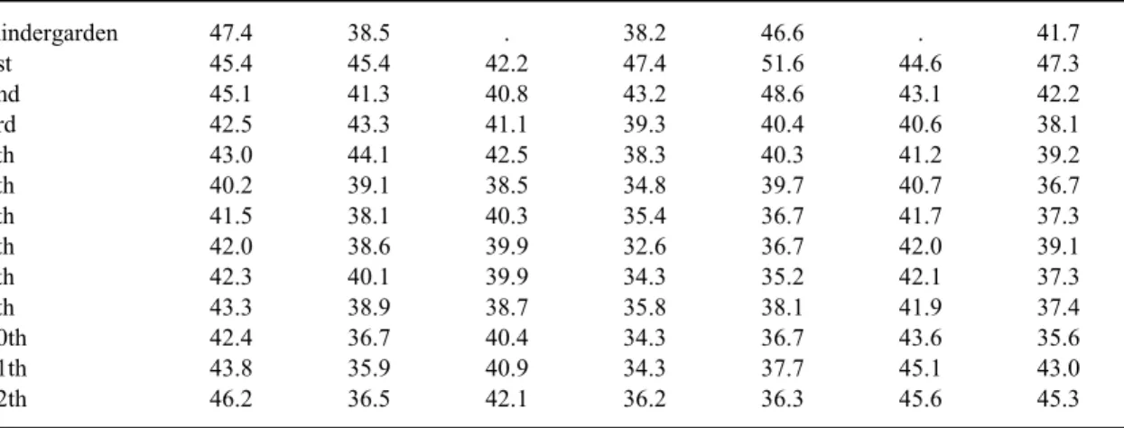
technical manuals for each test. Because it is the scaled scores that are comparable across grades, the effect sizes were computed from the mean scaled scores and the pooled standard deviations for each pair of adjacent grades.5_{The reading component of the California}

Achievement Test, 5th Edition (CAT/5), for example, has a spring national mean scaled score for kindergarten of 550, with a standard deviation of 47.4, and a first-grade spring mean scaled score of 614, with a standard deviation of 45.4. The difference in mean scaled scores — or growth — for the spring-to-spring transition from kindergarten to first grade is therefore 64 points. Dividing this growth by the pooled standard deviation for the two grades yields an effect size for the K-1 transition of 1.39 standard deviations. Calculations like these were made for all K-12 transitions for all tests and academic subject areas with available information.

Effect size estimates are determined both by their numerators (the difference be-tween means) and their denominators (the pooled standard deviation). Hence, the question will arise as to which factor contributes most to the grade-to-grade transition patterns found for these achievement tests. Because the standard deviations for each test examined are sta-ble across grades K-12 (Appendix Tasta-ble A.1) the effect sizes reported are determined al-most entirely by differences between grades in mean scaled scores.6_{In other words, it is the}

variation in growth of measured student achievement across grades K-12 that produces the reported pattern of grade-to-grade effect sizes, not differences in standard deviations across grades.7_{Indeed, the declining change in scale scores across grades is often noted in the}

technical manuals for the tests we examine, as is the relative stability of the standard devia-tions.8

The discussion below first examines the developmental trajectory for reading achievement based on information from the seven nationally normed tests. It then summa-rizes findings from the six tests of math, science, and social studies for which appropriate

5_{The pooled standard deviation is}

) 2 ( ) 1 ( ) 1 ( 2 2 − + − + − U L U U L L n n s n s n

, where L = lower grade and U = upper grade (for example, kindergarten and first grade, respectively).

6_{This is not the case for one commonly used test — the Iowa Test of Basic Skills (ITBS). Because its}

standard deviations vary markedly across grades and because its information is not available for all grades, the ITBS is not included in these analyses.

7_{Scaled scores for these tests were created using Item Response Theory (IRT) methods. Ideally, these}

measure “real” intervals of achievement at different ages, so that changes across grades do not also reflect differences in scaling. Investigation of this issue is beyond the scope of this paper.

8_{For example, the technical manual for}

TerraNova, The Second Edition: CAT, notes “As grade

in-creases, mean growth decreases and there is increasing overlap in the score distributions of adjacent grades. Such decelerating growth has, for the past 25 years, been found by all publishers of achievement tests. Scale score standard deviations generally tend to be quite similar over grades.” (2002, p. 235)

(19)

information was available. Last, the developmental trajectories are examined for two poli-cy-relevant subgroups — low-performing students and students who are eligible for free or reduced-price meals. The latter analysis is based on student-level data from a large urban school district.

Annual Reading Gains

Table 1 reports annual grade-to-grade reading gains measured as standardized mean difference effect sizes, based on information for the seven nationally normed tests examined for this analysis. The first column in the table lists effect size estimates for the reading component of the CAT/5. Note the striking pattern of findings for this test. Annual student growth in reading achievement is by far the greatest during the first several grades of ele-mentary school and declines thereafter throughout middle school and high school. For ex-ample, the estimated effect size for the transition from first to second grade is 0.97, the es-timate for grades five to six is 0.46, and the eses-timate for grades eight to nine is 0.30. This pattern implies that normative expectations for student achievement should be much greater in early grades than in later grades. Furthermore, the observed rate of decline across grades in student growth diminishes as students move from early grades to later grades. There are a few exceptions to the pattern, but the overall trend or pattern is one of academic growth that

declines at a declining rate as students move from early grades to later grades.

The next six columns in Table 1 report corresponding effect sizes for the other tests in the analysis. These results are listed in chronological order of the date that tests were normed. As can be seen, the developmental trajectories for all tests are remarkably similar in shape; they all reflect year-to-year growth that tends to decline at a declining rate from early grades to later grades.

To summarize this information across tests, a composite estimate of the develop-mental trajectories was constructed. This was done by computing the weighted mean effect size for each grade-to-grade transition, weighting the effect size estimate for each test by the inverse of its variance (Hedges, 1982).9_{Variances were computed in a way that treats}

9_{The variance for each effect size estimate is adapted from Equation 8 in Hedges (1982, p. 492):}

) ( 2 ˆ2 2 L i U i i L i U i L i U i i n n ES n n n n + + + =

σ

. The weighted mean effect size for each grade transition is adapted from Equation 13 in Hedges (1982, p. 494):

∑

= = = _k i i k i i i W ES ES 1 2 1 2 ˆ 1 ˆ σ σ

(20)

CAT/5 SAT 9 TerraNova CTBS Gates-MacGinitie MAT 8 TerraNova CAT SAT 10

Mean for the Seven Tests Grade K - 1 1.39 1.65 . 1.57 1.32 . 1.66 1.52 ± 0.21 Grade 1 - 2 0.97 1.08 0.89 1.18 0.91 0.82 0.95 0.97 ± 0.10 Grade 2 - 3 0.50 0.74 0.66 0.60 0.45 0.64 0.63 0.60 ± 0.10 Grade 3 - 4 0.40 0.53 0.26 0.54 0.29 0.24 0.24 0.36 ± 0.12 Grade 4 - 5 0.50 0.36 0.37 0.41 0.42 0.34 0.36 0.40 ± 0.06 Grade 5 - 6 0.46 0.24 0.23 0.34 0.34 0.17 0.45 0.32 ± 0.11 Grade 6 - 7 0.12 0.44 0.20 0.32 0.15 0.17 0.20 0.23 ± 0.11 Grade 7 - 8 0.21 0.30 0.23 0.27 0.30 0.26 0.25 0.26 ± 0.03 Grade 8 - 9 0.30 0.21 0.13 0.26 0.40 0.07 0.28 0.24 ± 0.10 Grade 9 - 10 0.16 0.19 0.20 0.20 0.04 0.21 0.32 0.19 ± 0.08 Grade 10 - 11 0.42 0.00 0.37 0.09 -0.06 0.34 0.20 0.19 ± 0.17 Grade 11 - 12 0.11 -0.05 0.12 0.20 0.04 0.11 -0.11 0.06 ± 0.11 Margin of Error (95%) Grade Transition Table 1

Annual Reading Gain in Effect Size from Seven Nationally Normed Tests

Achievement Effect-Size Benchmarks

SOURCES:

CAT/5 (1991 norming sample) and CAT/5 Technical Report, pp. 308-311.

SAT 9 (1995 norming sample) and SAT 9 Technical Data Report, Tables N-1 and N-4 (for SESAT), N-2 and N-5 (for SAT), and N-3 and N-6 (for TASK).

TerraNova CTBS (1996 norming sample) and Technical Report, pp. 361-366.

Gates-MacGinitie (1998-1999 norming sample) and Technical Report (Forms S and T), p. 57.

MAT 8 (1999-2000 norming sample), pp. 264-269. TerraNova CAT (1999-2000 norming sample) and Technical Report 1, pp. 237-242. SAT 10 (2002 norming sample) and Technical Data Report, pp. 312-338.

See References for complete citations.

NOTES: Spring-to-spring differences are shown. The mean is calculated as the random effects weighted mean of the seven effect sizes (five for the K-1 transition) using weights based on Hedges (1982). The K-1 transition is missing for the TerraNova CTBS and TerraNova CAT, because a "Vocabulary" component was not included in Level 10 of the test administered to K students. This component is included in the Reading Composite for all other grade levels.

(21)

estimated effect sizes for a given grade-to-grade transition as random effects across tests. This implies that each effect size estimate for the transition was drawn from a larger popu-lation of potential national tests. Consequently, inferences from the findings here represent a broader population of actual and potential tests of reading achievement.

The weighted mean effect size for each grade-to-grade transition is reported in the next to last column of Table 1. Reflecting the patterns observed for individual tests, this composite trajectory has larger effect size estimates in early grades, which decline by de-creasing amounts for later grades. The final column of the table reports the margin of error for a 95 percent confidence interval around each mean effect size estimate in the composite trajectory.10_{For example, the mean effect size estimate for the grade 1-2 transition is 0.97,}

and its margin of error is +0.10 standard deviation, resulting in a 95 percent confidence in-terval with a lower bound of 0.87 and an upper bound of 1.07.

Figure 1 illustrates the pattern of grade-to-grade transitions in the composite deve-lopmental trajectory for reading achievement tests. Weighted means are indicated by cir-cles, and their margins of error are represented by brackets around each circle. Also shown for each grade-to-grade transition is its minimum gain (as a diamond) and its maximum gain (as a triangle) for any of the seven tests examined. The figure thereby makes it possible to visualize the overall shape of the developmental trajectory for reading achievement of average students in the United States.

Ideally, this trajectory would be estimated from longitudinal data for a fixed sample of students across grades. By necessity, however, the estimates are based on cross-sectional data that, therefore, represent different students in each grade. Although this is (to our knowledge) the best information that exists for the purposes of this analysis, it raises a con-cern about whether cross-sectional grade-to-grade differences accurately portray

longitudin-al grade-to-grade growth. Cross-sectional differences will reflect longitudinal growth only

if the types of students are stable across grades (that is, student characteristics do not shift). For a large national sample, this is likely to be the case in elementary and middle school, which experience relatively little systematic student dropout. In high school, however, when students reach their state legal age to drop out, this could be a problem — especially in large urban school districts with high dropout rates.

To examine this issue, individual-level student data in which scores could be linked from year to year for the same students were used for two large urban school districts.These data were collected in an earlier MDRC study and enabled “head-to-head” comparisons of cross-sectional estimates of grade-to-grade differences and longitudinal estimates of grade-

(22)

12

to-grade growth. Longitudinal estimates were obtained by computing grade-to-grade growth only for students whose test scores were available for both the adjacent grades. For exam-ple, growth from first to second grade was computed as the difference between mean first-grade scores and mean second-first-grade scores for those students with both scores. The differ-ence between these means was standardized as an effect size using the pooled standard dev-iation of the two grades for the common sample of students. In cases where these data were available for more than one annual cohort of students for a given grade-to-grade transition, data were pooled across cohorts.11_{Cross-sectional effect sizes for the same grade-to-grade}

11_{For example, if first-grade and second-grade test scores were available for three annual cohorts of}

second-grade students, data on their first-grade tests were pooled to compute a joint first-grade mean (continued)

Figure 1

Mean Annual Reading Gain in Effect Size

-0.50 0.00 0.50 1.00 1.50 2.00 K-1 1-2 2-3 3-4 4-5 5-6 6-7 7-8 8-9 9-10 10-11 11-12 Ef fe c t S iz e Grade Transition

(23)

differences were obtained by comparing mean scores for all the students in a given grade (for example, first) to the mean scores for all the students in the next highest grade (for ex-ample, second) in the same school year (thus these were computed for different students). In cases where these data were available for more than one year, they were pooled across years. Table 2 presents the results of these analyses, showing for each district and for each grade transition the cross-sectional effect size, the longitudinal effect size, the difference in these two effects sizes, the difference in the difference of mean scores calculated cross-sectionally or longitudinally (as well its p-value threshold for a statistically significant dif-ference), and finally the standard error of the differences in difference of mean scores.

First, with one exception, the overall pattern of findings is the same for cross-sectional and longitudinal effect size estimates: Observed grade-to-grade growth for a par-ticular district tends to decline by declining amounts as students move from early grades to later grades. Second, for a particular grade transition in a particular district, there is no con-sistent difference between sectional and longitudinal estimates. In some cases, cross-sectional estimates are larger, and in other cases, longitudinal estimates are larger. Third, the magnitudes of differences between the two types of effect size estimates are typically small (less than 0.10 standard deviation). We do not conduct a direct test of the statistical significance of the difference between cross-sectional and longitudinal grade-to-grade effect size estimates. Instead, we assess this in terms of the difference between cross-sectional and longitudinal estimates of the grade-to-grade change in mean scaled scores.12_{As shown in}

the last two columns of Table 2, these differences are statistically significant at the 0.05 level in only one case (9-10 transition) for District I, but are more often statistically signifi-cant for transitions in District II. But even the differences that are statistically signifisignifi-cant are typically small in magnitude. Hence, the findings suggest evidence of small differences be-tween the cross-sectional and longitudinal effect size estimates.

The one striking exception to the preceding findings is the grade 9-10 transition. For this transition, cross-sectional estimates are much larger than longitudinal estimates in both school districts. They are also much larger than their counterparts in the national norming samples. This aberration suggests that in these districts, as students reach the legal age to drop out of school, those that remain in grade 10 are academically stronger that those who drop out. Except perhaps for the grade 9-10 transition, it thus appears that the

score, and data on their second-grade tests were pooled to compute a joint second-grade mean score. The joint standard deviation was computed as the square root of the mean of the within-year-and-grade va-riances involved, weighted by the number of students in each grade/year subsample.

(24)

14 Grade 1 - 2 District I 0.54 0.48 0.06 1.19 0.64 District II 0.97 0.93 0.05 2.07 ** 0.78 Grade 2 - 3 District I 0.41 0.39 0.02 0.39 0.71 District II 0.74 0.77 -0.03 -1.29 0.79 Grade 3 - 4 District I 0.70 0.64 0.06 1.55 0.81 District II 0.54 0.58 -0.05 -1.91 * 0.75 Grade 4 - 5 District I 0.40 0.44 -0.04 -1.02 0.90 District II 0.30 0.44 -0.14 -5.45 *** 0.67 Grade 5 - 6 District I 0.14 0.18 -0.04 -1.26 1.03 District II 0.15 0.34 -0.19 -7.23 *** 0.63 Grade 6 - 7 District I 0.37 0.34 0.03 0.82 1.03 District II 0.34 0.48 -0.15 -5.89 *** 0.71 Grade 7 - 8 District I 0.13 0.16 -0.03 -0.87 1.19 District II 0.33 0.39 -0.06 -2.30 *** 0.67 Grade 8 - 9 District I 0.07 0.15 -0.08 -2.77 1.47 District II 0.01 0.00 0.00 0.09 0.63 Grade 9 - 10 District I 0.66 0.42 0.25 8.97 *** 1.77 District II 0.36 0.08 0.28 11.09 *** 0.76 Grade 10 - 11 District I NA NA NA NA NA District II 0.20 0.07 0.13 5.21 *** 0.93

Table 2

Annual Reading Gain in Effect Size from School District Data:

Cross-Sectional Effect Size

Longitudinal Effect Size

Comparison of Cross-Sectional and Longitudinal Gaps in Two Districts

Grade Transition and District Difference in Difference of Mean Scores Standard Error of Difference in Difference of Mean Scores Difference in Effect Size

SOURCES: District I's outcomes are based on the Iowa Test of Basic Skills (ITBS) scaled scores for tests administered in spring 1997, 1998 and 1999, except for the grade 8-9 and 9-10 gaps, which are based on only the spring 1997 test results. District II's outcomes are based on SAT 9 scaled scores for tests administered in spring 2000, 2001 and 2002.

NOTES: Cross-sectional grade gaps are calculated as the average difference between test scores for two (continued)

(25)

sectional findings in Table 1 accurately represent longitudinal grade-to-grade growth in reading achievement for average U.S. students.13

Annual Math, Science, and Social Studies Gains

The analysis of the national norming data for reading described above was repeated using similar information for achievement in math, science, and social studies for six of the seven standardized tests.14_{Table 3 summarizes the results of these analyses alongside those}

for reading. The first column of the table reports the composite developmental trajectory (weighted mean grade-to-grade effect sizes) for reading; the next three columns report the corresponding results for math, science, and social studies.

The findings in Table 3 indicate that a similar developmental trajectory exists for all four subjects — average annual growth tends to decrease at a decreasing rate as students move from early grades to later grades. Not only is this finding replicated across all four subjects, but it is also replicated across the individual standardized tests within each subject (see Appendix Tables C.1, C.2, and C.3). Hence, the observed developmental trajectory ap-pears to be a robust phenomenon.

While the basic patterns of the developmental trajectories are similar for all four academic subjects, the mean effect sizes for particular grade-to-grade transitions vary noti-ceably. For example, the grade 1-2 transition has mean annual gains for reading and math

13_{Even the grade 9-10 transition might not be problematic for the national findings in Table 1. These}

cross-sectional effect size estimates do not differ markedly from those for adjacent grade-to-grade transi-tions. In addition, they are much smaller than corresponding cross-sectional estimates in Table 2 for the two large urban districts. Such differences suggest that high school dropout rates (and thus grade-to-grade student compositional shifts) are much less pronounced for the nation as a whole than for the two large urban districts in this analysis.

14_{This information was not available for the Gates-MacGinitie test.} Table 2 (continued)

grades in a given year. Longitudinal grade gaps are calculated as the average difference between a student's test score in a given year and that student's score one year later, regardless of whether the child was promoted to the next grade or retained. Students whose records show they skipped one or more grades in one year (for example, from grade 1 to 3) were excluded from the analysis because it was assumed that the data were in eror. These represented a very small number of records. Effect sizes are calculated as the measured gap divided by the unadjusted pooled student standard deviations from the lower and upper grades.

Statistical significance levels are indicated as *** = 0.1 percent; ** = 1 percent; * = 5 percent.

) 2 ( ) 1 ( ) 1 ( 2 2 − + − + − = U L U U L L n n s n s n pooledSD

(26)

16

(effect sizes of 0.97 and 1.03) that are markedly higher than those for science and social studies (0.58 and 0.63). On the other hand, for some other grade transitions, especially from sixth grade onward, these gains are more similar across subject areas.

Variation in Trajectories for Student Subgroups

Another relevant question is whether trajectories for student subgroups of particular interest follow the same pattern as those for average students nationwide. Figure 2 explores this issue based on student-level data from SAT 9 tests of reading achievement collected by MDRC for a past project in a large urban school district. Using these data, developmental trajectories were computed for three policy-relevant subgroups. One subgroup comprised all students in the school district (its student population). A second subgroup comprised students whose families were poor enough to make them eligible for free or reduced-price

Average Annual Gains in Effect Size for Four Subjects from Nationally Normed Tests

Reading Tests Math Tests Science Tests Social Studies Tests

Grade K - 1 1.52 1.14 NA NA Grade 1 - 2 0.97 1.03 0.58 0.63 Grade 2 - 3 0.60 0.89 0.48 0.51 Grade 3 - 4 0.36 0.52 0.37 0.33 Grade 4 - 5 0.40 0.56 0.40 0.35 Grade 5 - 6 0.32 0.41 0.27 0.32 Grade 6 - 7 0.23 0.30 0.28 0.27 Grade 7 - 8 0.26 0.32 0.26 0.25 Grade 8 - 9 0.24 0.22 0.22 0.18 Grade 9 - 10 0.19 0.25 0.19 0.19 Grade 10 - 11 0.19 0.14 0.15 0.15 Grade 11 - 12 0.06 0.01 0.04 0.04 Grade Transition

Table 3

SOURCES:

CAT/5 (1991 norming sample) and CAT/5 Technical Report, pp. 308-311.

SAT 9 (1995 norming sample) and SAT 9 Technical Data Report, Tables N-1 and N-4 (for SESAT), N-2 and N-5 (for SAT), and N-3 and N-6 (for TASK).

TerraNova CTBS (1996 norming sample) and Technical Report, pp. 361-366.

Gates-MacGinitie (1998-1999 norming sample) and Technical Report (Forms S and T), p. 57. MAT 8 (1999-2000 norming sample), pp. 264-269.

TerraNova CAT (1999-2000 norming sample) and Technical Report 1, pp. 237-242. SAT 10 (2002 norming sample) and Technical Data Report, pp. 312-338.

See References for complete citations.

NOTES: Spring-to-spring differences are shown. The mean for each grade transition is calculated as the weighted mean of the effect sizes from each available test. (See Appendix C.)

(27)

lunches. The third subgroup comprised students whose reading test scores were low enough to place them at the 25th percentile of their district.15_{Estimated effect sizes for each}

grade-to-grade transition for each subgroup are plotted in the figure as diamonds, triangles, or stars alongside those plotted for average students nationally (as circles).

These findings indicate that the shape of the overall trajectory for each subgroup in this district is similar to that for average students nationally: Annual gains tend to decline at a decreasing rate as students move from early grades to later grades. So once again, it ap-pears that the developmental pattern/trajectory identified by this analysis represents a robust phenomenon. Nonetheless, some variation exists across groups in specific mean annual gains, and other subgroups in other districts may show different patterns.

Implications of the Findings

The developmental trajectories presented above for average students nationally and for policy-relevant subgroups of students in a single school district describe normative growth on standardized achievement tests in a way that can provide benchmarks for inter-preting the effects of educational interventions. The effect sizes on similar achievement measures for interventions with students in a given grade can be compared with the effect size representation of the annual gain expected for students at that grade level. This is po-tentially a meaningful comparison when the intervention effect can be viewed as adding to students’ gains beyond what would have occurred during the year without the intervention.

For example, Table 1 shows that students gain about 0.60 standard deviation on na-tionally normed standardized reading achievement tests between the spring of second grade and the spring of third grade. Suppose a reading intervention is targeted to all third-graders and studied with a practice-as-usual control group of third-graders who do not receive the intervention. An effect size of, say, 0.15 on reading achievement scores for that intervention will, therefore, represent about a 25 percent improvement over the annual gain otherwise expected for third-graders. Figure 2 suggests that, if the intervention is instead targeted to the less proficient third-grade readers, the proportionate improvement may be somewhat less but not greatly different. That is a reminder, however, that the most meaningful comparisons will be with annual gain effect sizes from the specific population to which the in-tervention is directed. Such data will often be available from school records for prior years.

15_{For each grade, the district-wide 25th percentile and standard deviation of scaled scores were}

com-puted. These findings were then used to compute standardized mean effect sizes for each grade-to-grade transition for the 25th-percentile student.

(28)

18

The main lesson learned from studying the growth trajectories is that annual gains on standardized achievement tests — and hence any benchmarks derived from them — vary substantially across grades. Therefore, it is crucial to interpret an intervention’s effect in the context of expectations for the grade or grades being targeted. For example, suppose that the effect size for a reading intervention was 0.10. The preceding findings indicate that, rel-ative to normal academic growth, this effect represents a proportionally smaller improve-ment for students in early grades than for students in later grades.

It does not follow, however, that because a given intervention effect is proportional-ly smaller for earproportional-ly grades than for later grades it is necessariproportional-ly easier to produce in those early grades. It might be more difficult to add value to the fast achievement growth that oc-curs during early grades than to the slower growth that ococ-curs later. On the other hand,

stu-Achievement Effect-Size Benchmarks

Figure 2

Illustration of Variation in Mean Annual Reading Gain

-0.20 0.00 0.20 0.40 0.60 0.80 1.00 1.20 1.40 1.60 K-1 1-2 2-3 3-4 4-5 5-6 6-7 7-8 8-9 9-10 10-11 11-12 Ef fect Siz e Grade Transition

Mean Annual Gain Across Nationally Normed Tests Mean SAT 9 Gain for 1 District

Mean SAT 9 Gain for 25th-Percentile Students in 1 District Mean SAT 9 for Free/Reduced Lunch in 1 District

(29)

dents are more malleable and responsive to intervention in the earlier grades. What inter-vention effects are possible is an empirical question. Whatever the potential to affect achievement test scores, it may be informative to view the effect size for any intervention in terms of the proportion of natural growth it represents when attempting to interpret its prac-tical or substantive significance.

Another important feature of the findings presented above is that, while the basic patterns of the developmental trajectories are similar across academic subjects and student subgroups, the magnitudes of specific grade-to-grade transitions vary substantially. Thus, properly interpreting the importance of an intervention effect size requires doing so in the context of the type of outcome being measured and the type of students being observed. This implies that, although the findings in this paper can be used as rough general guide-lines, researchers should tailor their effect size benchmarks to the contexts they are studying whenever possible (the same point made by Cohen, 1988).

A final important point concerns the interpretation of developmental trajectories based on the specific achievement tests used for this analysis. These were all nationally normed standardized achievement measures for which total subject area scores were ex-amined. We do not necessarily expect the same annual gains in standard deviation units to occur with other tests, subtests of these tests (such as vocabulary, comprehension, etc.), or other types of achievement measures (such as grades or grade point averages, GPA). It is also possible that the developmental trajectories for the test scores used in our analyses re-flect characteristics distinctive to these broadband standardized achievement tests. Such tests, for instance, may underrepresent advanced content and thus be less sensitive to stu-dent growth in higher grades than in lower grades. Nevertheless, the tests used for the anal-ysis in this paper (and others like them) are often used to assess intervention effects in edu-cational research. The natural patterns of growth in the scores on such tests are therefore relevant to interpreting such effects, regardless of the reasons those patterns occur.

Benchmarking Against Policy-Relevant Performance Gaps

A second type of empirical benchmark for interpreting achievement effect sizes from educational interventions uses policy-relevant performance gaps among groups of stu-dents or schools as its point of reference. When expressed as effect sizes, such gaps provide some indication of the magnitude of the intervention effects that would be required to im-prove the performance of the lower-scoring group enough to help narrow the gap between the lower- and the higher-scoring group.

(30)

20

Because often “the goal of school reform is to reduce, or better, eliminate the achievement gaps between minority groups such as Blacks or Hispanics and Whites, rich and poor, and males and females…it is natural then, to evaluate reform effects by compar-ing them to the size of the gaps they are intended to ameliorate” (Konstantopoulos and Hedges, 2008, p. 1,615). While many studies evaluate such reforms (for example, Fryer and Levitt, 2006; Jencks and Phillips, 1998), very little work has focused on how to assess whether their effects are large enough to be meaningful.

This section builds on work by Konstantopoulos and Hedges (2008) to develop benchmarks based on observed gaps in student performance. One part of the analysis uses information from the National Assessment of Educational Progress (NAEP); the other part uses student-level data on standardized test scores in reading and math from a large urban school district. These sources of information make it possible to compute performance gaps, expressed as effect sizes, for key groups of students.

To calculate an effect size representing a performance gap between two groups re-quires knowledge of the means and standard deviations of their respective test scores. For example, published findings from the 2002 NAEP indicate that the national average fourth-grade scaled reading test score is 198.75 for black students and 228.56 for white students. The difference in means is therefore -29.81, which when divided by the standard deviation of 36.05 for all fourth-graders, yields an effect size of -0.83. The effect of an intervention that improved the reading scores of black fourth-grade students on an achievement test ana-logous to the NAEP by, for instance, 0.20 standard deviation, could then be interpreted as equivalent to a reduction of the national black-white gap by about one-fourth.

Findings from the NAEP

Table 4 reports standardized mean differences in reading and math performance be-tween selected subgroups of students who participated in the NAEP. Achievement gaps in reading and math scores are presented by students’ race/ethnicity, family income (free/reduced-price lunch status), and gender for the most recent NAEP assessments availa-ble at the time this paper was prepared. These assessments focus on grades 4, 8, and 12.16

All performance gaps in the table are represented in terms of effect size, that is, the differ-ence in mean scores divided by the standard deviation of scores for all students in a grade.

The first panel in Table 4 presents effect size estimates for reading. Within this pan-el, the first column indicates that at every grade levpan-el, black students have lower reading

16_{These NAEP gaps are also available for science and social studies, though not presented in this}

pa-per. In addition, performance gaps were calculated across multiple years using the Long-Term Trend NAEP data. These findings are available from the authors upon request.

(31)

scores than white students. On average, black fourth-graders score 0.83 standard deviation lower than white fourth-graders, with the difference decreasing slightly as students move to middle school and then to high school. The next two columns report a similar pattern for the gap between Hispanic students and white students, and for the gap between students who are eligible or not eligible for a free or reduced-price lunch. These latter gaps are smaller than the black-white gap but display the same pattern of decreasing magnitude with increas-ing grade level. The last column in the table indicates that mean readincreas-ing scores for boys are lower than those for girls in all grades. However, this gender gap is not as large as the gaps for the other groups compared in the table. Furthermore, the gender gap increases as stu-dents move from lower grades to higher grades, which is the opposite of the pattern exhi-bited by the other groups.

The second panel in Table 4 presents effect size estimates of the corresponding gaps in math performance. These findings indicate that at every grade level white students score higher than black students by close to a full standard deviation. Unlike the findings for read-ing, there is no clear pattern of change in gap size across grade levels (indeed there is very little change at all). Math performance gaps between Hispanic students and white students, and between students who are and are not eligible for a free or reduced-price lunch, are un-iformly smaller than corresponding black-white gaps. In addition, these latter groups exhibit a decreasing gap as students move from elementary school to middle school to high school

Black-White Hispanic-White Eligible-Ineligible for Free/

Reduced Price Lunch

Male-Female Reading Grade 4 -0.83 -0.77 -0.74 -0.18 Grade 8 -0.80 -0.76 -0.66 -0.28 Grade 12 -0.67 -0.53 -0.45 -0.44 Math Grade 4 -0.99 -0.85 -0.85 0.08 Grade 8 -1.04 -0.82 -0.80 0.04 Grade 12 -0.94 -0.68 -0.72 0.09

Subject and Grade

Demographic Performance Gap in Mean NAEP Scores, by Grade (in Effect Size)

Table 4

SOURCES: U.S. Department of Education, Institute of Education Sciences, National Center for Education Statistics, National Assessment of Educational Progress (NAEP), 2002 Reading Assessment and 2000 Mathematics Assessment.

(32)

22

(similar to the decreasing gap for reading scores). Lastly, the gender gap in math is very small at all grade levels, with boys performing slightly better than girls.

Konstantopoulos and Hedges (2008) found similar patterns among high school se-niors, using 1996 long-term trend data from NAEP. Among all demographic gaps ex-amined, the black-white gap was the largest for both reading and math scores. White stu-dents outperformed black stustu-dents and Hispanic stustu-dents; stustu-dents from higher socioeco-nomic status (SES) families outperformed those from lower SES families; males outper-formed females in math; and females outperoutper-formed males in reading.

Findings from a Large Urban School District

The preceding gaps for a nationally representative sample of students may differ from those of their counterparts in any given state or school district. To illustrate this point, Table 5 lists group differences in effect sizes for reading and math performance on the Stan-ford Achievement Test, Ninth Edition (SAT 9), taken by students in a large urban school district.17_{Gaps in reading and math scores are presented by students’ race/ethnicity,}

free/reduced-price lunch status, and gender for grades 4, 8, and 11, comparable to the na-tional results in Table 4.

The first panel in Table 5 presents effect size estimates for reading. The findings in the first column indicate that, on average, white students score about one standard deviation higher than black students at every grade level. Findings in the second column indicate sim-ilar results for the Hispanic-white gap. Findings in the third column indicate a somewhat smaller gap based on students’ free or reduced-price lunch status, which unlike the race/ethnicity gaps, decreases as students move through higher grades. Findings in the last column indicate that the gender gap in this school district is quite similar to that nationally in the NAEP. Males have lower average reading scores than females, and this difference increases with increasing grade levels.

The second panel in Table 5 presents effect size estimates for math. Again, on aver-age, white students score about one standard deviation higher than black students at every grade level, with the gap increasing in the higher grades. The pattern and magnitude of the gap between Hispanic and white students is similar, whereas the gap between students who are and are not eligible for a free or reduced-price lunch is smaller than the corresponding race/ethnicity gaps and, like reading, decreases from elementary to middle to high school. Finally, the gender gap is much smaller than that for other student characteristics, with

17_{District outcomes are based on average SAT 9 scaled scores for tests administered in spring 2000,}

(33)

males having higher test scores than females in the upper grades, but not in the fourth-grade.

Implications of the Findings

The findings in Tables 4 and 5 illustrate a number of points about empirical bench-marks for assessing intervention effect sizes based on policy-relevant gaps in student per-formance. First, suppose the effect size for a particular intervention was 0.15 on a standar-dized achievement test of the sort analyzed above. The findings presented here indicate that this effect would constitute a smaller substantive change relative to some academic gaps (for example, between blacks and whites) than for others (for example, between males and females). Thus, it is important to interpret a study’s effect size estimate in the context of its target groups of interest.18

A second implication of these findings is that policy-relevant gaps for demographic subgroups may differ for achievement in different academic subject areas (here, reading and math) and for different grades (here, grades 4, 8, and 11 or 12). Thus, when interpreting an intervention effect size in relation to a policy-relevant gap, it is important to make the

18_{This point does not imply that it is necessarily easier to produce a given effect size change to close}

the gaps for some groups than for others.

Black-White Hispanic-White Eligible-Ineligible for Free/

Reduced Price Lunch

Male-Female Reading Grade 4 -1.09 -1.03 -0.86 -0.21 Grade 8 -1.02 -1.14 -0.68 -0.28 Grade 11 -1.11 -1.16 -0.58 -0.44 Math Grade 4 -0.95 -0.71 -0.68 -0.06 Grade 8 -1.11 -1.07 -0.58 0.02 Grade 11 -1.20 -1.12 -0.51 0.12

Subject and Grade

Table 5

Demographic Performance Gap in SAT 9 Scores from a Selected School District, by Grade (in Effect Size)

SOURCE: MDRC calculations from individual students' school records for a large, urban school district. NOTE: District local outcomes are based on SAT 9 scaled scores for tests administered in spring 2000, 2001, and 2002.

(34)

24

parison for the relevant outcome measure and target population. Third, benchmarks derived from local sources (such as school district data) may provide more relevant guidance than findings from national data for interpreting effect sizes for interventions in that local con-text.

An important caveat with regard to using policy-relevant gaps in student perfor-mance as effect size benchmarks is that it may be important to periodically reassess them. For example, Konstantopoulos and Hedges (2008) found that, from 1978 to 1996, achieve-ment gaps between blacks and whites and between Hispanics and whites decreased in both reading and math. During the same period, the gender gap increased slightly for reading and decreased for math.

Benchmarking Against Differences among Schools

Performance differences between schools may also be relevant for policy, as school reform efforts are typically designed to make weak schools better by bringing them closer to the performance levels of average schools. Or, as Konstantopoulos and Hedges put it, because some “school reforms are intended to make all schools perform as well as the best schools….it is natural to evaluate reform effects by comparing them to the differences (gaps) in the achievement among schools in America” (2008, p. 1,615). Thus, another poli-cy-relevant empirical benchmark refers to achievement gaps between schools, and in par-ticular, “weak” schools compared with “average” schools.

To illustrate the construction of such benchmarks, we used individual student achievement data in reading and math to estimate what the difference in achievement would be if an “average” school and a “weak” school in the same district were working with com-parable students (that is, those with the same demographic characteristics and past perfor-mance). We defined average schools to be those at the 50th percentile of the school

perfor-mance distribution in a given district, and we defined weak schools to be those at the 10th percentile of this distribution.

Calculating Achievement Gaps Between Schools

School achievement gaps were measured as effect sizes standardized on the student-level standard deviation for a given grade in a district. The mean scores for 10th- and 50th-percentile schools in the effect size numerator were estimated from the distribution across schools of regression-adjusted mean student test scores. The first step in deriving these es-timates was to fit a two-level regression model of the relationship between present student test scores for a given subject (reading or math) and student background characteristics, in-cluding a measure of their past test scores. Equation 1 illustrates such a model.

Performance Trajectories and Performance Gaps as Achievement Effect-Size Benchmarks for Educational Interventions