STR profile authentication via machine learning techniques

Short Tandem Repeat (STR) Profile

Authentication via Machine Learning Techniques

by

Anna Shcherbina

Submitted to the Department of Electrical Engineering and Computer

Science

in partial fulfillment of the requirements for the degree of

Master of Engineering in Computer Science and Engineering

at the

MASSACHUSETTS INSTITUTE OF TECHNOLOGY

May 2012

@

Massachusetts Institute of Technology 2012. All rights reserved.

A u th or ...

Department of Electrical Engineering and Computer Science

May 21, 2Q12

Certified by...

. ..

a p d l

S r4 Anhony Lapadula

MIT Lincoln Laborat r Technical Staff

/hpis

Sypervisor

Certified by...

Accepted by ...

z:::

VKanolis Kellis

Associate Professor

Thesis Supervisor

Prof. Dennis M. Freeman

Chairman, Masters of Engineering Thesis Committee

Short Tandem Repeat (STR) Profile

Authentication via Machine Learning

Techniques

by

Anna Shcherbina

Submitted to the Department of Electrical Engineering and

Computer Science

on May 21, 2012, in partial fulfillment of the

requirements for the degree of

Master of Engineering in Computer Science and Engineering

Abstract

Short tandem repeat (STR) DNA profiles have multiple uses in forensic analysis, kinship identification, and human biometrics. However, as biotechnology progresses, there is a growing concern that STR profiles can be created using standard laboratory techniques such as whole genome amplification and molecular cloning. Such technolo-gies can be used to synthesize any STR profile without the need for a physical sample, only knowledge of the desired genetic sequence. Therefore, to preserve the credibility of DNA as a forensic tool, it is imperative to develop means to authenticate STR profiles. The leading technique in the field, methylation analysis, is accurate but also expensive, time-consuming, and degrades the forensic sample so that further analysis is not possible.

The realm of machine learning offers techniques to address the need for more effec-tive STR profile authentication. In this work, a set of features were identified at both the channel and profile levels of STR electropherograms. A number of supervised and unsupervised machine learning algorithms were then used to predict whether a given STR electropherogram was authentic or synthesized by laboratory techniques. With the aid of the LNKnet machine learning toolkit, various classifiers were trained with the default set of parameters and the full set of features to quantify their base-line performance. Particular emphasis was placed on detecting profiles generated by Whole Genome Amplification (WGA).

A greedy forward-backward search algorithm was implemented to determine the most useful subset of features from the initial group. Though the set of optimal feature values varied by classifier, a trend was observed indicating that the inter-locus imbalance error, stutter count, and range of peak widths for a profile were particularly

useful features. These were selected by over two thirds of the classifiers. The signal-to-noise ratio was also a useful feature, selected by seven out of 16 classifiers.

The selected features were in turn used to tune the parameters of machine learning algorithms and to compare their performance. From a set of 16 initial classifiers, the K-nearest neighbors, condensed K-nearest neighbors, multi-layer perceptron, Parzen window, and support vector machine classifiers achieved the best performance. These classification algorithms all attained error rates of approximately ten percent, defined as the percentage of profiles misclassified with the highest performing classifier achiev-ing an error rate of less than eight percent. Overall, the classifiers performed well at detecting artificial profiles but had more difficulty accurately distinguishing natu-ral profiles. There were many false positives for the artificial class, since profiles in this category took on a greater range of feature values. Finally, preliminary steps were taken to form classifier committees. However, combining the top performing classifiers via a majority vote did not significantly improve performance.

The results of this work demonstrate the feasibility of a completely software-based approach to profile authentication. They confirm that machine learning techniques are a useful tool to trigger further investigation of profile authenticity via more ex-pensive approaches.

Thesis Supervisor: Dr. Anthony Lapadula Title: MIT Lincoln Laboratory Technical Staff Thesis Supervisor: Manolis Kellis

Title: Associate Professor

This work is sponsored by the Assistant Secretary of Defense for

Research and Engineering under Air Force Contract FA8721-05-C-0002. Opinions, interpretations, conclusions and recommendations are those of the authors and are not necessarily endorsed by the United States

Acknowledgments

First and foremost I want to thank my supervisor at Lincoln Laboratory, Dr. Anthony Lapadula. Thank you for providing mentorship and advice throughout my thesis research. Your help and support has been invaluable, and I appreciate your many great ideas that have helped me overcome sticking points over the course of my research. I would also like to thank Dr. Martha Petrovick and Johanna Bobrow for providing the raw STR profile data needed for my research and suggesting features to examine in the feature identification phase of the project. I am also extremely grateful to Edward Wack, group leader of the Biological Engineering Group at MIT Lincoln Laboratory, for accepting me into the group and enabling the funding of my MEng work.

Additionally, I would like to thank Professor Manolis Kellis, my MEng advisor at MIT, for providing great suggestions about machine learning algorithms and tech-niques. I have learned a lot about the application of machine learning techniques to problems in biology by speaking to you about my thesis work and taking your course on computational biology.

I would furthermore like to thank the staff who run the VI-A program for pro-viding such an amazing opportunity for students like me to obtain valuable industry experience while completing an MEng degree.

Finally, I would like to thank my parents, Tatyana Proshko and Yuri Shcherbina, for working extremely hard to give me extensive opportunities in education and more generally in life. Thank you for encouraging me to pursue my academic interests and for providing emotional (and financial) support as I navigated the frequently uncertain waters of my education at MIT.

Contents

1 Short Tandem Repeat (STR) Profiles: Natural and Synthetic

Ap-proaches 19

2 Data Analysis 25

2.1 Source STR Profile Availability ... 25

2.2 Profile Acquisition ... ... 26

2.3 Extracting Electropherogram Information from .fsa Files . . . . 29

2.4 Feature Identification . . . . 30

2.5 Feature Granularity/Establishing Patterns for Classification . . . . . 36

2.6 High Level Feature Analysis . . . . 37

3 Machine Learning Algorithms for STR Profile Classification 41 3.1 Classifier Training: Developing Accurate Discriminant Functions Be-tw een C lasses . . . . 42

3.2 N-Fold Cross Validation . . . . 43

3.3 Classifier Taxonomy . . . . 46

3.4 Improving Classifier Performance . . . . 50

4 Feature Selection 51 4.1 Replicate Analysis . . . . 52

4.3 Clustering Algorithms . . . . 56

4.4 Effects of Feature Selection . . . . 57

5 Parameter Optimization 61 5.1 Motivation for Parameter Tuning . . . . 61

5.2 Parameter Tuning Algorithm . . . . 63

5.3 Performance Evaluation . . . . 64

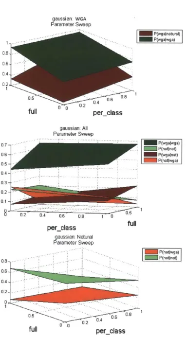
5.4 Parameter Tuning Examples for the Gaussian and ARTmap classifiers 65 5.5 Full Parameter Sweeps . . . . 71

6 Results of Feature Selection and Parameter Tuning: Determining Optimal Classifier Behavior 75 6.1 Classifier Comparison with Performance Score Weights [1,1,1,1,1] 75 6.2 High-Performing Classifiers . . . . 78

6.2.1 K-Nearest Neighbors (KNN) . . . . 78

6.2.2 Condensed K-Nearest Neighbors (CKNN) . . . . 79

6.2.3 Multi-Layer Perceptron (MLP) . . . . 80

6.2.4 Parzen W indow . . . . 85

6.2.5 Support Vector Machine (SVM) . . . . 87

6.3 Emphasis on Minimizing False Negatives for WGA Class . . . . 88

6.4 Emphasis on Correctly Classifying Natural vs. Correctly Classifying W G A . . . . 92

6.5 Machine Learning on the PowerPlex STR Typing Kit . . . . 98

6.6 Distinguishing Natural Profiles from Bacterial Clones . . . . 100

7 Committee Classifiers 105 7.1 Committee Generation by Stacking . . . . 106

7.1.1 Majority Vote Results . . . . 107

7.1.3 Average of Classifier Results . . . . 110

7.1.4 Median of Classifier Results . . . . 112

7.2 Random Forest . . . . 114

8 Project Extensions 119 8.1 Classifier Committees via Boosting . . . . 119

8.2 M ulti-Class Classification . . . . 120

8.3 Identify the Source of Classifier Errors . . . . 120

8.4 Determining ROC Curves . . . . 121

8.5 Other Cost Metrics: Time and Memory . . . . 121

8.6 Quantitative Estimate of Classifier Generalization . . . . 123

9 Summary of Major Conclusions 125

A Raw Feature Data for Identifiler Kit 131

B Features Selected by a Variety of Classifiers 139

C Individual Classifier Tuning 147

D Combined Classifier Performance as a Function of Scoring Weights

and Feature Optimization Parameters 157

List of Figures

1-1 Each person inherits two alleles at an STR locus, one from each parent.

The two alleles can differ in the number of base pair repeats. . . . . . 20

1-2 Bacterial cloning summary. For purposes of this project, the pink strands of "foreign DNA" refer to DNA segments that contain the

CODIS loci and Amelogenin [24]. . . . . 22

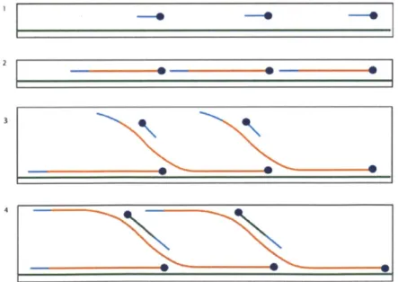
1-3 Whole genome amplification (WGA). (1) The random hexamers (rep-resented by a blue line) bind to the denatured DNA (rep(rep-resented by a green line). (2) The DNA polymerase (represented by a blue circle) extends the primers until it reaches newly synthesized double-stranded DNA (represented by an orange line). (3) The enzyme proceeds to displace the strand and continues the polymerization, while primers bind to the newly synthesized DNA. (4) Polymerization starts on the

new strands, forming a hyper-branched structure [11]. . . . . 22

2-1 Two cycles of PCR are illustrated. The red and orange lines represent the DNA template to which primers (pink and green ovals) anneal. [19]. 26 2-2 AmpFLSTR Identifiler allelic ladder (Applied Biosystems). A total of

205 alleles are included in this ladder used for genotyping a multiplex PCR reaction involving 15 STR loci and the amelogenin sex-typing test. 28

2-3 A natural profile obtained via multiplexed PCR with the Identifiler kit. The alleles of interest are indicated by fluorescence peaks. The size standard, in the bottom channel, was aligned with the size standard from a ladder. The aligned sample was then compared with the ladder

to identify allele peaks based on their size. . . . . 30

2-4 Sample natural STR profile from Identifiler kit with 4 Channels, 16 Loci, and a size standard. Boxed values represent called alleles. . . . 31

2-5 Intra-locus imbalance. . . . . 32

2-6 Differences in intensity between natural and WGA profiles are noted with the blue and red circles. A drop-in allele is present in the WGA (lower) channel. . . . . 33

2-7 Ski slope and stutter peaks. . . . . 35

2-8 Peak shape and signal-to-noise ratio. . . . . 35

2-9 Split peaks due to incomplete adenylation do not follow the expected Gaussian shape [5]. . . . . 36

3-1 The training phase of classifier development involves creating a dis-criminant function that forms decision boundaries between the natural and WGA classes in multi-dimensional space. . . . . 44

3-2 K-fold cross validation was used to combat low data availability by using each profile for both training and testing [42]. Four folds were used (K = 4). . . . . 45

3-3 Classifier approaches to forming decision regions

[35].

3-4 Machine learning classifier development overview. . . . . 50

4-1 A natural profile with four replicates. . . . . 53

4-3 Support vector machine feature selection. The results of feature

selec-tion for other classifiers are included in Appendix B. . . . . 55

4-4 Identifiler profile misclassification pre- and post- feature selection. Fea-ture selection led to a drop of 13 percentage points in the overall

num-ber of classification errors. . . . . 58

4-5 Some features are particularly useful across a variety of the classifiers

exam ined. . . . . 59

5-1 The covariance matrix of a Gaussian classifier can be calculate in four

w ays [38]. . . . . 62

5-2 The performance of the Gaussian classifier depends on its covariance

m atrix [38]. . . . . 63

5-3 Gaussian classifier with parameters full, per-class . . . . 67

5-4 Fuzzy ARTmap classifier schematic [24]. . . . . 68

5-5 Artmap classifier with parameters alpha test- vigil, alpha-train-vigil,

al-pha, beta, beta-vigil. . . . . 70

5-6 Parameter sweep for the Gaussian classifier with covariance matrix

determined by parameters full and per-class. . . . . 72

5-7 Parameter sweep tuning for the ARTmap classifier with parameters

alpha-train vigil, alpha-test vigil, and beta. . . . . 73

6-1 Identifiler, weights =[1,1,1,1,1], column 1: default performance,

col-umn 2: performance after feature selection, colcol-umn 3: performance

after parameter tuning. . . . . 76

6-2 Identifiler, weights =[1,1,1,1,1]. Performance after parameter tuning

is show n . . . . 76

6-3 K nearest neighbors with parameter K. . . . . 79

6-5 _{Multi-layer perceptron with parameters epochs, alpha, nodes, etta, etta-change-type,}

hfunction, ofunction, cost-fun, init-mag, sigmoid-param. . . . 83

6-5 (continued). . . . . 84

6-6 _{Parzen classifier with parameters per-input, per-class, minvar, spread,}

lin ear. . . . . 86

6-7 SVM classifier with parameters sigma and cbound. . . . 88

6-8 Identifiler, weights = [1,1,1,10,1]. p(natlwga) was assigned a cost 10 times higher than any other error. Column 1: default performance,

column 2: feature selection, column 3: parameter tuning. . . . . 90

6-9 Identifiler, weights = [1,1,1,10,1], tuned parameters. p(natlwga) was

assigned a cost 10 times higher than other errors. . . . . 90

6-10 Identifiler, weights =[1,1,1,1,1] compared with weights [1,1,1,10,1]. . 92

6-11 Identifiler, weights = [3,1,1,3,1], features optimized for natural profile

classification. . . . . 96

6-12 Identifiler, weights = [1,3,3,1,1], features optimized for WGA profile

classification. . . . . 96

6-13 Identifiler, comparison between classifiers optimized for identifying nat-ural profiles (weight vector [3,1,1,3,1]), and classifiers optimized for

identifying WGA (weight vector [1,3,3,1,1]). . . . . 97

6-14 PowerPlex, natural vs WGA, weights =

[1,1,1,1,1],

performance, column 2: performance after feature selection, column 3:

performance after parameter tuning. . . . . 99

6-15 PowerPlex, natural vs. WGA, weights = _{[1,1,1,1,1]. Performance after}

param eter tuning. . . . . 99

6-16 PowerPlex, natrual vs. bacterial cloned/synthetic, weights = [1,1,1,1,1],

column 1: default performance, column 2: feature selection, column 3:

6-17 PowerPlex, natural vs bacterial, tuned parameters, weights =

[1,11,1,11].102

6-18 Parameters optimized, weights =[1,1,1,1,1. The three columns in

each bar represent Identifiler natural vs. WGA, PowerPlex natural vs.

WGA, PowerPlex natural vs. bacterial. . . . . 103

7-1 Majority vote committees. . . . . 107

7-2 Majority vote committee test data misclassifications. . . . . 108

7-3 Natural profile that was classified as WGA by all six majority vote

com m ittees. . . . . 109

7-4 Natural profile that was classified correctly by all six majority vote

com m ittees. . . . . 109

7-5 Majority Vote of Five Top-Performing Classifiers: CKNN, KNN, MLP,

Parzen, SVM . . . .111

7-6 Committees formed by averaging individual classifier results. . . . . . 112

7-7 Mean committee test data misclassifications. . . . . 113

7-8 Committees formed by taking the median of individual classifier results. 113

7-9 Median committee test data misclassifications. . . . . 114

7-10 Random forest out-of-bag error: individual trees compared with

cumu-lative forest. . . . . 117

8-1 Method to generate receiver operating characteristic (ROC) curve [43]. 122

8-2 A single layer of the MLP algorithm on a separable data set can be implemented via logical "and", "or", "majority" functions, which all return correct outputs, but differ in training and test time

[35]

exam ined. . . . . 126

9-2 Identifiler, weights =[1,1,1,1,1], features optimized, column 1: baseline performance, column 2: feature selection, column 3: parameter tuning. 128

9-3 Identifiler, weights = [1,1,1,1,1], fine-tuned parameters. . . . . 128

A-I Gaussian Error For Each Channel and Profile (Normalized, No Outliers) 132 A-2 Heterozygote Intralocus Imbalance For Each Channel and Profile (Nor-m alized, No Outliers) . . . . 132

A-3 Interchannel Intensity For Each Channel and Profile (Normalized, No O utliers) . . . 133

A-4 Interlocus Imbalance Error For Each Channel and Profile (Normalized, N o O utliers) . . . 133

A-5 Interchannel Intensity For Each Channel and Profile (Normalized, No O utliers) . . . 134

A-6 Off Ladder Inside Bin For Each Channel and Profile (Normalized, No O utliers) . . . 134

A-7 Off Ladder Outside Bin For Each Channel and Profile (Normalized, N o O utliers) . . . 135

A-8 Peak Width For Each Channel and Profile (Normalized, No Outliers) 135 A-9 Ski Slope For Each Channel and Profile (Normalized, No Outliers) . . 136

A-10 SNR For Each Channel and Profile (Normalized, No Outliers) . . . . 136

A-11 Stutter Count For Each Channel and Profile (Normalized, No Outliers) 137 B-1 Artmap Classifier Feature Selection . . . 140

B-2 Bintree Classifier Feature Selection . . . 140

B-3 Condensed K Nearest Neighbors Classifier Feature Selection . . . 141

B-4 Gaussian Classifier Feature Selection . . . 141

B-5 Gaussian Mixture Model Feature Selection . . . 142

B-6 Histogram Classifier Feature Selection . . . 142

B-7 Hypersphere Classifier Feature Selection . . . 143

B-9 K Nearest Neighbors Classifier Feature Selection . . . . 144

B-10 Linear Vector Quantizer Classifier Feature Selection . . . . 144

B-11 Multi-Layer Perceptron Feature Selection . . . . 145

B-12 Naive Bayes Classifier Feature Selection . . . . 145

B-13 Nearest Cluster Classifier Feature Selection . . . . 146

B-14 Parzen Classifier Feature Selection . . . . 146

C-1 Binary Tree Classifier with parameters leaf-minnpatterns, prune-val, m ax-node. ... . ... . .. . . . .. . . . .. . . . . .. .. . . . 148

C-2 Gaussian Mixture Classifier with parameters grand, full, var-spread, epochs... ... 149

C-3 Histogram Classifier with parameters grand-bins, bintype, nbins, range-factor. 150 C-4 Hypersphere Classifier with parameters grand-bins, bintype, nbins, range-factor. . . . . 151

C-5 Incremental Radial Basis Function with parameters fclparam, weight eta, max-magnitude, bias, grand, cost-fun . . . . 152

C-6 Learning Vector Quantizer with parameters epochs, alpha, lvqtype, w indow , epsilon . . . . 153

C-7 Naive Bayes Classifier with parameters range-factor, bins. . . . . 154

C-8 Nearest Cluster Classifier with parameters fclparam, gauss-dist, minvar. 155 C-9 Radial Basis Function with parameters hspread-default, exhspread-default, fclparam-default, maxratio-default, minvar-default, bias-default. . . . 156

D-1 Identifiler, weights =[1,1,1,1,1], features optimized for "natural" . 158 D-2 Identifiler, weights =[1,1,1,1,1], features optimized for "wga" . . . . . 158

D-3 Identifiler, weights = [1,1,1,10,1], features optimized for "natural" 159

D-4 Identifiler, weights = [1,1,1,10,1], features optimized for "wga" . 159

D-6 Identifiler, weights = [1,2,2,1,1], features optimized for "wga" . . . . . 160 E-1 Gaussian Error For Each Channel and Profile (Normalized, No Outliers) 162 E-2 Heterozygote Intralocus Imbalance For Each Channel and Profile

(Nor-m alized, No Outliers) . . . . 162

E-3 Interchannel Intensity For Each Channel and Profile (Normalized, No

O utliers) . . . . 163

E-4 Interlocus Imbalance Error For Each Channel and Profile (Normalized,

N o O utliers) . . . . 163

E-5 Interchannel Intensity For Each Channel and Profile (Normalized, No

O utliers) . . . . 164

E-6 Off Ladder Inside Bin For Each Channel and Profile (Normalized, No

O utliers) . . . . 164

E-7 Off Ladder Outside Bin For Each Channel and Profile (Normalized,

N o O utliers) . . . . 165

E-8 Peak Width For Each Channel and Profile (Normalized, No Outliers) 165

E-9 Ski Slope For Each Channel and Profile (Normalized, No Outliers) . . 166

E-10 SNR For Each Channel and Profile (Normalized, No Outliers) . . . . 166

List of Tables

2.1 Data availability by profile type and test kit. . . . . 25

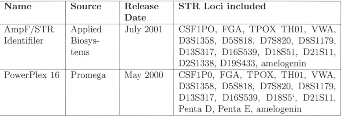
2.2 Commercially available STR multiplexes used to analyze STR profiles. 28

2.3 Identification of features at the channel level. . . . . 38

3.1 Machine learning algorithms used to train profile classifiers

[7].

4.1 Feature guide: each number indicates a specific feature value for a profile. 60

6.1 Performance of top classifiers: CKNN, SVM, KNN, MLP, Parzen. . . 77

6.2 _{Comparison of classifier performance with w=[1,1,1,1,1] and [1,1,1,10,11}

by profile category. . . . . 92

6.3 Comparison of classifier performance with w=[3,1,1,3,1] and [1,3,3,1,1]

by profile category. . . . . 98

7.1 Six committees were formed by taking different combinations of

indi-vidual classifiers. In addition to the five committees presented, a sixth

committee was formed by taking a majority vote of all the classifiers. 106

7.2 Majority vote among high-performing classifiers: CKNN, KNN, MLP,

Parzen, SV M . . . . 110

7.3 Standard deviation in out-of-bag error for individual trees and forests. 116

9.1 Feature guide: each number indicates a specific feature value for a

Chapter 1

Short Tandem Repeat (STR)

Profiles: Natural and Synthetic

Approaches

Eukaryotic genomes contain many repeated sequences. These vary in size, and are typically identified by the length of the core repeat unit and the number of adjacent repeat units. Alternatively, they can also be designated by the overall length of the repeat region and fall into three categories: long repeat units with several hundred to several thousand bases in the core repeat are referred to as satellite DNA; medium-length repeat units with 10-100 bases in the repeat region are called minisatellites; finally, DNA regions with repeat units that are 2-6 base pairs in length are termed microsatellites, or short tandem repeats (Figure 1-1).

Thousands of polymorphic microsatellites have been characterized in human DNA, and there may be more than a million microsatellite loci present [12]. These mark-ers are scattered throughout the genome and occur roughly every 10,000 nucleotides, jointly comprising approximately 3% of the human genome [13]. STRs are of particu-lar interest in human identification and have become a popuparticu-lar DNA marker because

Human Chromosomes

MO" EA:A TG] AATG

Mel

7 Rapew

8 Repeat

Figure 1-1: Each person inherits two alleles at an STR locus, one from each parent. The two

alleles can differ in the number of base pair repeats.

they are short and can consequently be easily amplified by the polymerase chain reaction (PCR) with minimal problems caused by differential amplification. Small product sizes are also compatible with degraded DNA, and PCR enables recovery of information from small amounts of material. Additionally, the number of repeats in STR markers is highly variable among individuals, making combinations of STR alleles particularly effective for human identification.

The thirteen loci included in the National DNA Index System (NDIS) are of particular interest for forensics and human identification. NDIS is a DNA database funded by the United States Federal Bureau of Investigation (FBI) that stores DNA profiles created by federal, state, and local crime laboratories in the United States. The associated software, the Combined DNA Index System (CODIS), provides the ability to search the database to assist in the identification of criminal suspects. The 13 loci in the NDIS database provide the bulk of the loci analyzed in this work.

These are CSF1PO, FGA, TH01, TPOX, VWA, D3S1358, D5S818, D7S820, D8S1179, D13S317, D16S539, D18S51, and D21S11. For the full set of 13 loci, the probability of a random match in the profiles of two unrelated individuals is less than one in a trillion [20]. By generating STR profiles that also include Amelogenin (used to determine gender) and two additional loci specific to individual multiplex PCR kits, the random match probability can be further reduced. By October 2008, NDIS had grown to include over 241, 685 forensic profiles and 6, 384, 379 offender profiles [3].

Many techniques exist to generate synthetic STR profiles, such as bacterial cloning and whole genome amplification (WGA). These are summarized in Figures 1-2 and 1-3 respectively. These and other techniques can be performed using equipment

com-monly available in Biosafety Level 1 (BL1)1 and Biosafety Level 2 (BL2)2 labs. This

project focuses primarily on whole genome amplification, with a brief extension to bacterial cloning. Qiagen, the manufacture of a commercials WGA kit, claims that this process is unbiased and that a WGA profile should be indistinguishable from a natural one. However, frequently this is not the case. Quantifying the Qiagen am-plified DNA with the Identifiler kit, for example, revealed that WGA underestimates the amount of DNA present.

Currently, bisulfite sequencing is the state-of-the art technique used to authen-ticate STR profiles. This technique involves performing methylation analysis of the profile in question, based on the concept that human DNA is methylated but bacterial DNA is not [25]. This is effective because most methods to produce artificial DNA employ bacteria as a tool to amplify desired sequences. However, bisulfite sequencing leads to 90% degradation of the DNA due to the need for long incubation times, high temperatures, and elevated bisulfite concentrations. Furthermore, this technique is

'This level is suitable for work involving well-characterized agents not known to consistently cause disease in healthy adult humans, and of minimal potential hazard to laboratory personnel and

the environment [2].

2

This level is similar to Biosafety Level 1 and is suitable for work involving agents of moderate potential hazard to personnel and the environment. It includes various bacteria and viruses that cause only mild disease to humans, or are difficult to contract via aerosol in a lab setting [2].

ForeignDNA

S rPlasnd EcoRI eoointerest

resistance EcoRI Ec.R~ EcaRIEcR Sticky ends Hybridbuation + DNA Ugase Recombina DNA DNA insertion

Bacteia acterial Bacteria platted on medium

cell6R omosome + anibotic

ciaug

__ _ _

Only bacteria containing recombinant DNA vrow

Culture CloneDNA

Cloning into a plasmid

Figure 1-2: Bacterial cloning summary. For purposes of this project, the pink strands of 'foreign

DNA" refer to DNA segments that contain the CODIS loci and Amelogenin [24].

2

-0--3

4F

pM

Figure 1-3: Whole genome amplification (WGA). (1) The random hexamers (represented by a

blue line) bind to the denatured DNA (represented by a green line). (2) The DNA polymerase (represented by a blue circle) extends the primers until it reaches newly synthesized double-stranded

DNA (represented by an orange line). (3) The enzyme proceeds to displace the strand and continues

the polymerization, while primers bind to the newly synthesized DNA. (4) Polymerization starts on the new strands, forming a hyper-branched structure [11].

expensive and time-consuming.

The shortcomings of bisulfite sequencing suggest the usefulness of a software-based approach based on machine learning models trained on low-cost, readily available STR profiles. Thus, machine learning algorithms provide a valuable tool to detect the bias introduced by WGA and other means of STR profile generation. Although the conclusions inferred by these algorithms should not serve as a definitive test, they provide a useful trigger to run more conclusive and costly tests.

Chapter 2

Data Analysis

2.1

Source STR Profile Availability

Genetic data was obtained in accordance with COUHES protocols from buccal swabs of volunteer donors. Since Identifiler kit data for WGA and natural samples was most readily available, the majority of the analysis was performed on the datasets in the "Identifiler Test Kit" column of Table 2.1. The low availability of data for the

Identifiler Test Kit PowerPlex 16 Test Kit

Natural 1 Sample, 4 Replicates 10 Samples, 1 Replicate

40/40 Unique Samples 16 Samples, 0 Replicates

23 Samples, 1 Replicate

WGA 1 Sample, 4 Replicates 5 Samples, 1 Replicate

58/5 Unique Samples 25 Samples, 0 Replicates

35 Samples, 1 Replicate

Bacterial (Cloned) 1 Sample, 16 Replicates

Bacterial (Synthetic) 1 Sample, 16 Replicates

Table 2.1: Data availability by profile type and test kit.

bacterial samples in the PowerPlex kit (one unique bacterial clone and one unique sample synthesized from scratch) suggests that machine learning algorithms trained on the bacterial PowerPlex samples should be verified on larger datasets. For many of the donors in the study, several STR profiles were obtained. Thus, "1 sample, 4

replicates" means that one unique donor's profile, plus four additional profiles from the same donor, were obtained for purposes of analysis. See Chapter 4 for a more detailed discussion of replicate samples.

2.2

Profile Acquisition

STR profiles were obtained via the multiplexed polymerase chain reaction (PCR), a rapid way of amplifying specific DNA sequences (Figure 2-1). PCR was performed by adding the DNA to be amplified to a solution containing short tandem primers, the four nucleotides, and DNA polymerase. Three steps were then performed iteratively until a sufficient quantity of the desired sequence has been generated: (1)the DNA was denatured at 94-96 'C. (2) annealed to primers at 65 'C(3) elongated at 72 'C. Using this process, it is possible to obtain billion-fold amplification (32 cycles of PCR) in one hour [19]. The 13 CODIS loci, the amelogenin sex-typing marker, and two additional STR loci were co-amplified in a single reaction using existing commercial primer sets.

95 dog

mmom

4M1

DNA Synthsis

4 4

Figure 2-1: Two cycles of PCR are illustrated. The red and orange lines represent the DNA template to which primers (pink and green ovals) anneal. [19].

The samples were then subjected to parallel analysis via capillary electrophoresis using an Applied Biosystems 3130 genetic analyzer (AB13130) [41]. The AB13130

used amplicon sizing to identify individual alleles. Based on the analysis kit used, different fluorescent dyes were attached to PCR primers that were incorporated into the amplified target region of the source DNA. Amplified STR alleles were represented by peaks in an electropherogram.

One or more allelic ladders were included in each batch of STR profiles analyzed with the AB13130. An allelic ladder is an artificial mixture of the common alleles present in the human population for a particular STR marker [9]. Such allelic ladders serve as a standard for each STR locus (see Figure 2-2). These ladders are generally created with the same primers as test samples and provide a reference DNA size for each allele. They are used to adjust for different sizing measurements obtained from different runs of the AB13130 instrument. Ladders are constructed by combining locus-specific PCR products from multiple individuals in a population. The samples are then co-amplified to produce an artificial sample containing the common alleles for the STR marker. The allele quantities are balanced by adjusting the input amount of each component so that the alleles are fairly equally represented in the ladder. Internal standards labelled with a different color from the STR alleles were used to perform the DNA size determinations and subsequent correlation with an allelic ladder to obtain an STR genotype.

The rapid processing and multiplex capabilities of the ABI3130 genetic analyzer encourage the development of machine learning techniques to authenticate the output of this technique. For example, both 96-well and 384-well plates of samples can be processed with the ABI 3130. With each run taking 45-60 minutes, a 96-well plate can be analyzed in approximately 5-6 hours [9]. These capabilities make multiplex PCR analysis of STR profiles more attractive to forensics and biometrics laboratories in comparison to more expensive and time-consuming approaches such as methylation analysis.

instru-Ladder for AmpF/STR Identfier Kit (Appled Biosystems) 0801170 300 40820 3179 C00 50 0 15000 - 12ANe2 . aa 1 11s ,so I ~ LI' 1, I ' , u I JI ~00 3500 000 4000 4500 500 5500 6000 6500 7000 fVels (1008

(70moho. 77(0 ile) 9a8s) (1 .5le)

39)00 3500 4000 4500 5000 5500 600 650 7000

Figure 2-2: AmpFLSTR Identifier allelic ladder (Applied Biosystems). A total of 205 alleles are included in this ladder used for genotyping a multiplex PCR reaction involving 15 ST R loci and the

amelogenin sex-typing test.

Name Source Release STR Loci included

Date

AmpF/STR Applied July 2001 CSF1PO, FGA, TPOX TH01, VWA,

Identifiler Biosys- D3S1358, D5S818, D7S820, D8S1179,

tems D13S317, D16S539, D18S51, D21S11,

D2S1338, D19S433, amelogenin

PowerPlex 16 Promega May 2000 CSF1P0, FGA, TPOX, TH01, VWA,

D3S1358, D5S818, D7S820, D8S1179, D13S317, D16S539, D18S5', D21S11,

Penta D, Penta B, amelogenin

Table 2.2: Commercially available STR multiplexes used to analyze STR profiles.

ment because of their widespread usage in the forensics and biometrics communities (Table 2.2). Both kits amplify the 13 CODIS loci/amelogenin and are able to iden-tify repeat lengths within similar size ranges. The primary differences between them lie in the additional loci analyzed (Penta E and Penta D for PowerPlex 16; D2S1338 and D19S433 for Identifiler). Additionally, the two kits differ in their dye-labelling

strategies: the PowerPlex 16 kit uses four dyes (three channels and a size standard), while the Identifiler kit uses five dyes (four channels and a size standard). A third

difference is in the size standards used: ILS600 CXR for PowerPlex 16 and GS500 LIX for Identifiler.

2.3

Extracting Electropherogram Information from

.fsa Files

The AB13130 Genetic Analyzer stores STR profile data in the .fsa format. A Python module was developed to convert the data to human-readable format, extract signals for further analysis, and obtain relevant information about the electrophoresis process. Code was written to identify the fluorescence value of each channel in the electropherogram as a function of scan number (a measure of time). Timestamps for each channel were used to identify the associated ladder. Multiple ladders were included with each PCR sample to account for variations in experimental conditions (i.e. changes in temperature, photo-bleaching) that could effect allele resolutions and introduce artifacts into the STR profile. Consequently, each channel within a profile was analyzed with respect to the nearest ladder. This custom code makes use of the ABIFReader Python module published by Interactive Biosoftware [5,41].

The signals obtained from the files were then processed in MATLAB to identify allele values for each locus, locate off-ladder alleles, and extract feature values for each sample.Peak alignment techniques were used to overlay the size standard in the bottom channel of an electropherogram over the size standard of the associated allelic ladder. This was done to align the allele peaks in the ladder with corresponding allele peaks in the individual sample and identify the allele value for each locus. An example of a resulting STR profile is presented in Figure 2-3. A series of steps was then performed to identify feature values for the sample. The individual features of interest are summarized in Section 2.4, and Figure 2-4 demonstrates an example of an STR profile with annotated alleles and feature values.

Natural Profile Obtained via Identifiler Kit DBS1179 1179 D21Si D7 0 CSFPO .3 3000 0 3504000 T. I 4500 500550060060 I A 103S3 D13S317~~~383s3 4 D2S133 1 1338 430 000 4500 5000 5500 6000 6500 200 1000 019S433 D19S433 VWA VWA TPX T151 3000 3500 4500 5000 5500 6000 6500 2000 L'

1000o -~ 053818 D5S818 FGA FGA

3000 3500 4000 45 5000 5500 6000 6500 0 100 - 1 0 0 p 139b101bp p 200hp 25 5 p 30bp 34-p * 3000 3500 4000 4500 5000 550 6000 6500 Scan Number

Figure 2-3: A natural profile obtained via multiplexed PCR with the Identifiler kit. The alleles of

interest are indicated by fluorescence peaks. The size standard, in the bottom channel, was aligned with the size standard from a ladder. The aligned sample was then compared with the ladder to identify allele peaks based on their size.

2.4

Feature Identification

Having obtained annotated STR profile from the MATLAB processing pipeline, the next step was to identify features useful for distinguishing between natural and artificial profiles. These features in combination served as the raw material on which to train a suite of machine learning algorithms to perform authentication. Prior research and examination of the data led to the identification of eleven features. Many of these were based on common biological artifacts of STR markers, such as stutter products, non-template nucleotide addition, microvariants, null alleles, and

mutations. The full set of 11 analyzed features included:

* Intra-locus imbalance: Ratio of peak heights between the alleles in a single heterozygous locus (Figure 2-5). Intra-locus peak height ratios were calculated for a given locus by dividing the peak height of an allele with a lower fluorescence intensity (shorter peak) by the peak height of an allele with a higher intensity (taller peaks). Theoretically, two alleles for an individual who is heterozygous

Natural_01_004_D01 2000

F

IA

-

_I

--L

F

0

r1

Figure 2-4: Sample natural STR profile from Identifiler kit with ~4 Channels, 16 Loci, and a size

at a single locus should be present in equal amounts in the genome, amplify equally, and have peak heights are that are approximately equal, with a peak height ratio near 1. In practice, intra-locus imbalance may occur if the DNA source is inhibited, degraded, preferentially amplified, or subject to unequal sampling of true alleles [42]. The latter two conditions are more likely to occur in a laboratory-synthesized profile, suggesting the use of this feature to distinguish between natural and synthetic samples.

Intralocus Balance: Ratio of minor peak height to major peak height at heterozygous loci

Scanumber

Figure 2-5: Intra-locus imbalance.

9 Inter-locus imbalance: Ratio of peak heights among adjacent loci in an

elec-tropherogram. This feature was calculated in two ways. The first approach involved computing the ratio of tallest locus to shortest locus in a channel. The second approach involved finding the mean squared error between each individual locus and the mean intensity for the channel.

0 0 C

* Fluorescence intensity: Measured by peak height (see Figure 2-6).

* Frequency and position of off-ladder alleles: STR microvariants are rare alleles that result from point mutations or insertion/deletions of a block smaller than the locus repeat block size. An off-ladder outside bin allele is a microvariant that does not correspond to any of the standard STR loci included in a test kit (Identifiler/PowerPlex 16); an off-ladder inside bin allele corresponds to a stan-dard locus but does not match any of the stanstan-dard alleles for that locus [28].

Natural and artificial samples were compared for the presence of both kinds of microvariants. See Figure 2-6 for an example of a drop-in allele in a sample profile. The feature analysis techniques used to annotated profiles were able to detect allele drop-in, but not allele drop-out, which causes a heterozygous sam-ple to look like a homozygous samsam-ple. The feature identification protocol could be extended to accommodate allele dropout by obtaining STR profiles with both the Identifiler and PowerPlex 16 test kits and comparing the heterozygosity of each peak.

Intensity and Drop-in Allele

i.:

II

-~J

Two channels of afour-chamel electrophetogran

Drop In

WsA-Scan iumbe

Figure 2-6: Differences in intensity between natural and WGA profiles are noted with the blue and

" Frequency and position of stutter peaks: Stutter product peaks are small peaks that differ in size from an allele peak by one or two repeat units. Stutter products are caused by slip-strand mispairing of the DNA polymerase during replication. Insertion, caused by slippage of the copying strand, leads to a stut-ter product one repeat unit longer than the main allele. Deletion, caused by slippage of the copied strand, causes a stutter product one repeat unit shorter than the main allele. Since different polymerases are used in natural and syn-thetic DNA replication, and use of faster polymerase results in fewer stutter products, it is possible that the frequency and position of stutter peaks may differ between natural and artificial samples. Typically, a stutter product is 5-15% of the height of the adjacent allele peak [28]. In Figure 2-7, stutter peaks are denoted by small golden dots located near the baseline.

" Ski slope: Biological samples become degraded when exposed to adverse en-vironmental conditions. Since degradation breaks the DNA at random, larger amplified regions are affected first and the height of the peaks in an electrophero-gram decreases from left to right (Figure 2-7). Since artificial DNA samples are less likely to be subject to adverse environmental conditions, it is possible that the ski slope may be a distinguishing feature between the two classes [16]. * Presence of pull-up: Pull-up occurs when the analysis software is unable to

discriminate between the different dye colors used for sequencing. If matrix color deconvolution in the fluorescence analysis process does not work properly, a color may bleed from one spectral channel into another, usually because of off-scale peaks

[1].

" Signal to noise ratio: The peaks were interpreted as the signal; any non-relevant disturbances in the baseline were interpreted as noise. Figure 2-8 illustrates the higher noise observedfor some WGA profiles relative to natural profiles.

M1Ski Slope

t

f

tf

-- t

3000 4000 50O 6000 700

Figure 2-7: Ski slope and stutter peaks.

Natural

I I

WGA

410F 4112 41 sno

Figure 2-8: Peak shape and sigqnal-to- noise ratio.

* Peak shape/area: In natural DNA, peak shape closely approximates a Gaussian curve. Additionally, the peak distribution has a predictable pattern based on the extraction method used and the extent of DNA degradation. Variations in peak shape may be observed due to phenomena such as non-template addition [1]. In the process of adenylation, the Taq polymerase adds an extra adenine nucleotide to the end of a PCR product. Depending on the 5' end of the reverse primer, a guanine can be added to the end of a primer to promote non-template addition. Excess amounts of DNA template in a PCR reaction can result in incomplete adenylation due to insufficient quantities of polymerase, which can be observed on an STR profile as a split peak (Figure 2-9). Since this phenomenon depends

___

Incomplete

adenylation

+A +A

-A ,A

D8S1 179

Figure 2-9: Split peaks due to incomplete adenylation do not follow the expected Gaussian shape [51.

on both the amount of DNA present and the polymerase used to replicate the DNA, it is possible that the frequency of incomplete adenylation is different for WGA and natural profiles.

2.5

Feature Granularity/Establishing Patterns for

Classification

The full set of feature values was calculated for each profile with the goal of combining many weak trends to build an accurate profile classifier. The optimal feature granularity was determined experimentally. In one approach, individual peaks served as the patterns for classifications, and feature values were calculated for every peak. For example, the intra-locus imbalance for a peak was found by calculating the ratio of the two peak heights in a heterozygous allele. This ratio was assigned as the intra-locus imbalance for both peaks in the locus. For homozygotes, the intra-locus imbalance was set to one for the single peak in the locus. When each peak was treated as a separate classification pattern with a full set of feature values, the data shortage problem was avoided, since each sample had a high number of peaks. However, some features, such as ski slope and inter-locus imbalance, are not defined for individual peaks, but rather for combinations of peaks. Multiple peaks must thus be assigned the same feature value. For example, all peaks in a channel would be assigned the

same value for the ski slope feature. This approach functions like a smoothing filter and leads to loss of information about the data.

Consequently, to avoid bias, channels were used as patterns for classification rather than individual peaks. Table 2.3 presents the formulas used to calculate each feature at the channel level. After features were calculated at the channel level, profile statis-tics were obtained. For each profile, the minimum, maximum, mean, and range of the feature values across the individual channels were calculated. For example, com-puting the ski slope for the channels in an Identifiler profile results in four values, one for each channel. The minimum of these four is defined as the profile minimum, the maximum among the four is the profile maximum, the difference between the max-imum and minmax-imum is defined as the range of the ski slope feature for the profile, and the mean of the four values is the profile mean. Empirically, examining features at the profile level through the min, max, mean, and range statistics led to slightly reduced error rates in the baseline classifier performance (mean reduction 2% across all the classifiers examined). Consequently, all subsequent analysis was performed at the profile level. That is, each sample had 44 unique features - a profile minimum, maximum, mean, and range for each of the 11 features listed in Table 2.3.

2.6

High Level Feature Analysis

Once features had been identified and computed for each of the natural, WGA, and bacterial profiles, a high level analysis was performed of the resulting distribu-tions. The scatter plots in Appendix A and Appendix E show the feature values for the Identifiler and PowerPlex datasets, respectively. The blue dots represent nat-ural profiles, while the red dots represent WGA. In each subplot there are 87 red dots and 37 blue dots, indicative of the 87 WGA and 37 natural profiles that were analyzed with the Identifiler kit. The green dots in Appendix E represent bacterial profiles (bacterial clones and synthetic samples were analyzed jointly). The process used to generate the bacterial clones is discussed in Chapter 1, Figure 1-2. Although

fea-p

E

Value

across locus intensity

(locus intensity - p)2 E (E)2 E3 Me"aMloMs Es EL intensity

]ZIEI

signal-to-noise ratio _{A=locus intensity average}

a-non-peak variance 0 0 00 Feature Value Feature inter-locus imbalance error

(E channel peak widths) (E profile peak widths)

Gaussian er- E(error)2 _{over all peaks}

ror in channel

ski slope

off-ladder count

outside bin

off-ladder in- count side bin

stutter count

Best &t wrs

LALLLALk

Table 2.3: Identification of features at the channel level.

Notes/Clarification

" All channel features are propagated to the profiles as Min, Max, Range, Average * Locus intensity = E (Peak Intensity at Locus)

Locus 0 Intensity

Peak Intensity

ture values were computed for the bacterial dataset, only one bacterial clone and one bacterial synthetic profile was available for study. Consequently, additional data must

heterozyote * geometric mean over all

intra-locus heterozygous loci

imbalance * 1 if all loci in channel

are homozygous

inter-locus ratio of locus intensity

imbalance (Max:Min)

ratio peak width

be gathered to draw solid conclusions about feature selection for bacterial profiles and to train high-performing classifiers (Table 2.1).

Figure A-2 provides an illustrative example of differences in feature values be-tween natural and WGA profiles. The figure illustrates intra-locus imbalance values for each profile. The top row illustrates the intra-locus imbalance value of the four individual channels, while the bottom subplot shows the minimum, maximum, range, and mean of the intra-locus imbalance for the profile. In each of the eight subplots, the WGA datapoints are more spread out than the natural. The blue natural feature values cluster near 0.9, but the red WGA values have no significant clusters. Rather, they are spread fairly uniformly through the range of valid intra-locus imbalance val-ues, from zero to one. This trend is highly evident at the channel level (top row). It is weaker at the profile level: the range and mean values for both WGA and natural profiles are spread throughout the [0-1] range. However, the natural data is more clustered than the WGA data for the profile min and max.

This observation can be generalized for the majority of the features examined. For nearly each feature plot in Appendix A, the WGA profiles take on a higher range of values, with a correspondingly higher standard deviation. This phenomenon influences classifier performance and is discussed in Chapter 6. The higher spread of feature values for WGA profiles results in a high incidence of false positives for the WGA class, that is, natural profiles misclassified as WGA. Since WGA profiles can take on a greater variety of feature values, classifiers are more likely to mark a profile as WGA than natural. Thus, careful feature selection is necessary to discover the subset of features for each classifier to minimize both false positives and false negatives.

Chapter 3

Machine Learning Algorithms for

STR Profile Classification

Once a set of features had been identified to differentiate between natural and syn-thetic STR profiles, as described in Chapter 2, these features were used as inputs to a set of machine learning algorithms. The algorithms operate on the principle that a learner can use example data to identify relationships between observed feature vectors. A major focus of machine learning research is to automatically learn to rec-ognize complex patterns and make intelligent decisions based on data; the difficulty lies in the fact that the set of all possible behaviors given all possible inputs is too large to be covered by the set of observed examples (training data). Consequently, the learner must generalize from the given examples, so as to be able to produce a useful output in new cases (test data).

Machine learning classifiers are trained by partitioning data into two groups: train-ing and test. If sufficient data is available, a third evaluation group may also be created. A classification algorithm uses the training data set to learn the difference between the classes. The evaluation set, if present, is used to evaluate classifier per-formance and to determine whether further training is necessary. Ultimately, the

classification algorithm computes a set of parameters that form a discriminant func-tion between the two classes. Given a new profile, the algorithm applies this funcfunc-tion

to classify it.

The pattern classification approach is particularly relevant to STR profile authen-tication for several reasons. First, this approach works well for noisy, complex, or unknown processes, and there is a high level of noise and complexity in the acquired STR profile data. Furthermore, pattern classification is particularly appealing when features can be measured and training data is available, both of which are conditions that hold for the STR profile sample set [38].

3.1

Classifier Training: Developing Accurate

Dis-criminant Functions Between Classes

A classifier consists of a discriminant function that is constructed during the

train-ing phase. This function consists of a linear combination of feature values multiplied

by weights w (Figure 3-1). It has the following mathematical form:

D

y(x) = f( Xi * wi)

i=O

e x refers to the input feature vector. In Chapter 2, 44 distinct features were identified, so the feature vector for each sample STR profile consists of 44 values.

" w is the vector of coefficients that produce the desired characteristics in the

discriminant function. The focus of the training phase is to optimize this weight vector so that the function y takes on dissimilar values for input samples that belong to different classes and similar values for inputs that belong to the same class.

" D is the number of features used to train the classifier. It is equal to 44 for the

* f refers to the function that governs the behavior of the machine learning al-gorithm. Step functions, linear separators, and sigmoids area all commonly used by classification algorithms. Binary trees, support vector machines, and Gaussian mixture models respectively implement these functions. Examples are illustrated in Figure 3-1.

The discriminant function takes a feature vector as an input and projects this vector into a higher-dimensional feature space. This feature space is partitioned by decision boundaries, and an input feature vector is classified based on the location of the projection relative to these boundaries [40]. For example, the right half of Figure 3-1 illustrates the projection of two input feature vectors (A and B) onto a

two-dimensional space defined by features x1 and x2. Since one vector is projected

above the decision boundary and the other one is projected below the boundary, the two vectors get assigned to different classes.

Training a classifier consists of performing discriminant analysis to find the optimal

vector of weights w. At each iteration the current discriminant function is used

to project the input data to a high-dimensional feature space and to classify them according to their position relative to a set of decision boundaries. The algorithm then

identifies training samples that were misclassified. The weight vector w is updated

to reduce the number of misclassifications in future iterations. The exact manner in which this vector is updated is algorithm-specific. When the number of misclassified training data samples drops below a pre-defined threshold, training is complete and the weight vector is fixed at its current value. The classifier is said to be trained.

3.2

N-Fold Cross Validation

Due to the small sample sizes for both the Identifiler and PowerPlex test kits, there was insufficient data to split the profiles into training, evaluation, and test sets. To deal with the scarcity of data, four-fold cross validation was performed to select

Training a Classifier Discriminant Function

44 Input Features

<x1 x2, x3,-..X 4 4>

'I

o =1 I w. Compute Discriminant

X, Output Function y for Each Class

e-y(x) V(x) = ZxA t 1ai a +1 m m +1 H AR 0 (AR 0 G -1 -i -1

HARD LUMITER LUNEAR SIGMOID

I

Decision

"Natural"

or

"WGA"

Figure 3-1: The training phase of classifier development involves creating a discriminant function that forms decision boundaries between the natural and WGA classes in multi-dimensional space.

features and tune parameters for individual classifiers [42]. The advantage of the cross validation technique is that all available samples were used as both test objects and training objects. To perform four-fold cross validation, samples were separated into four folds, and each was tested against a classifier trained on the data in the other three folds (Figure 3-2). The error rates from the individual test folds were summed to obtain the overall error rate of the classifier.

As demonstrated in Figure 3-2, classifier training and evaluation via four-fold cross validation can be summarized as follows:

YWGA I

Select Maximum y (2D Example)

Classification Rule

Class Natural if y>=O Class WGA if y <0