MACHINE
LEARNING
APPLICATIONS
IN
MORTGAGE
DEFAULT PREDICTION
Bolarinwa Akindaini
University of Tampere
Faculty of Natural Sciences M.Sc. thesis
Supervisor: Martti Juhola November 2017
I
University of Tampere Faculty of Natural Sciences
Master’s Degree Programme in Computational Big Data Analytics Machine Learning Applications in Mortgage Defaults Predictions M.Sc. thesis, 55 pages
November 2017
Abstract
Estimating default risk has been a major challenge in credit-risk analysis. Financial institutions are interested in the ability of a customer to payback a loan. In this research work we explore the application of some machine learning models in the prediction of mortgage defaults. We basically explore how machine learning methods can be used to classify mortgages into paying, default and prepay. This work examines the following machine learning methods: Logistic regression (simple and multi-class), Naive Bayes, Random forest and K-Nearest Neighbors. Finally, this work includes Survival analysis and Cox proportional hazard rate to estimate the probability of loan survival pass certain time and the impact of each variable in estimating the probability of survival respectively.
Key words and terms: Machine Learning, Default, Prepaid, Hazard model, Survival analysis.
II
Contents
1 Chapter One 1
1.1 Introduction 1
1.2 Literature Review 2
1.3 Data Sources and Description 4
Chapter Two 6
2.1 Exploratory Analysis 6
2.2 Variable Description 12
Chapter Three 14
3.1 Logistic Regressions 15
3.1.1 Simple Logistic Regression 16
3.1.2 Multi-class Multinomial Logistic Regression 23
3.2 Naive Bayes Classifier 27
Chapter Four 30
4.1 Random Forest Model 30
4.2 KNN Model 35
4.3 Survival Analysis and Cox Proportional Hazard Model 39
4.3.1 Survival Analysis 39
4.3.2 Cox Proportional Hazard Model 42
Chapter Five 49
5.1 Summary and Conclusion 49
1
1 Chapter One
1.1 Introduction
Mathematically, mortgages have been judged as one of the most complex securities. These complexities are because of many factors some of which include: the repayment options available to homeowners, the ability to capture fully the behavior of mortgages in different states of the world, in-homogeneity of loan level behaviors, and the fact that single period analysis cannot be used for path-dependent instruments such as mortgages. It is also interesting to note that the behavior of a single loan may vary under different economic situations. Similarly, different loan types behave differently under same economic situations.
One of the ways to assess the strength of a financial institution is to evaluate the performance of the organization’s loan portfolio loss during stressed situation by estimating the chances of default (i.e. the probability that a loan will go into default or not). This step is quite important for risk management and credit risk analysis.
In the early 1980’s, mortgage default was basically evaluated by rules of thumb and credit risk ratings based on professional experience. The rating was done by using four variables: debt to income ratio (DTI), monthly repayment to income ratio, loan to value ratio (LTV), and house value to income ratio. These methods of credit risk appraisal provided a certain degree of default risk; however, this was insufficient for two reasons. Firstly, the quantitative assessment of the probability of default cannot be determined by risk ratings. Secondly, these methods failed to consider the timing of default as they basically focus on the likelihood or the probability of default during the active period of the mortgage. Later on, traditional econometric models such as linear regression and generalized linear regression were employed to evaluate mortgages for defaults. These methods mainly focused on finding causality for specific predictors that followed certain theoretical knowledge. The results of these models were mainly presented in terms of the statistical significance of predictors with R-squared ratio but the results were hardly analyzed in terms of out-of-sample accuracy. On the other hand, machine learning is a relatively new concept in financial modelling. However, machine learning
2
methods allow quantitative assessment of defaults, analyzing results in terms of out-of-sample accuracy by specifying test sets and training sets, and lastly assessing the timing of defaults.
In 2007, the increase of subprime mortgages led to a wide range of financial crises, the resulting effect was a high rate of defaults on mortgages. Prior to this, non-government agencies were in charge of mortgage backed securities market and most mortgages followed the guidelines laid down by Fannie Mae and Freddie Mac. Later there was a bubble in the market which was sensitive to consumers’ expectations and economic fluctuations. This bubble was as a result of non-government agencies loosening the guidelines and rules that governed the mortgages.
This thesis focuses on applying machine learning methods to explore and predict the outcome of a single-family loan (default, prepaid, and paying) by using data published by Fannie Mae. We start with an exploratory analysis of the dynamic variables to determine variables to be included in the model in chapter two and then presented the following parametric models in chapter three: Simple logistic, Multi-class multinomial logistic regression and Naive Bayes. In chapter four, the nonparametric models which include KNN model and Random forest model were introduced and applied to the dataset. Since the time of occurrence of each of the classification outcome is of great importance to financial institutions, we conclude chapter four by presenting Survival analysis and Cox proportional hazard model. In chapter five, the entire work was briefly summarized, and recommendations made.
1.2 Literature Review
Application of machine learning in finance is a relatively new concept and as such related literatures are quite few. However, research relating to the analysis of mortgage defaults and credit risk are in good numbers. The earliest study of the analysis of defaults in commercial mortgages was carried out by Magee (1968). Later in 1969, von Furstenberg did a comprehensive study of the impact of loan age and loan-to-value ratio on mortgage default rates. He then concluded his work in 1970 by stating that these two
3
variables were the major factors in determining default rates in mortgages. Subsequently, additional variables were examined by Vandell (1978) and Gau (1978). Gau’s work was based on finding empirical factors that influence defaults and prepayment rates. He postulated that in determining default covariates, the ratio of loan value to the property value could be used. Curley and Guttentag (1974) used simulation and sensitivity analysis to judge the impact of prepayment probabilities on expected future cash flows. The impact of interest rates on prepayments and defaults was examined by Green & Shoven (1986). Prior to Green & Shoven (1986) study, Campbell & Dietrich (1983) had done a study to analyze the determinants of default and prepayment for insured residential mortgages using a multinomial logit model for cross-sectional and time series data. Recent studies on the analysis of mortgage default include Capozza (1997), Ambrose & Deng (2001) and LaCour-Little and Malpezzi (2003). The first two studies were aimed at verifying the impact of low down payments and fallen house prices on default rates while the last study considered the impact of the direct selling price on default rate.
It is interesting to note that these previous studies were based on small sample data. The invention of software that can easily handle very large amounts of data has made the application of machine learning more interesting. Hence our study is a clear shift from the previous studies because our data consist of nearly 45 million loans and approximately about 2.8 billion observations all estimated at about $10 trillion. Previous studies considered dataset in the range of thousands with emphasis on specific geographical locations. The dataset used in this work covers all states and cities in the United States with adequate representation of all geographical locations in each city. Two new variables unemployment rate and rent-ratio were included to capture macroeconomic fluctuations within the period under review.
Machine learning has been extensively studied in different fields (e.g speech recognition, pattern recognition, image classification, and natural language processing). Similarly, machine learning has been employed to predict defaults in consumer and commercial loans. Such studies include Khandani, Kim & Lo (2010), Butaru, Chen, Clark, Das, Lo & Siddique (2015), Pericli & Hu (1998), Feldman & Gross (2005), and Fitzpatrick & Mues (2016). However, this work is quite different from these studies
4
because we focus on the worst-case scenario of 90 days default for subprime mortgages and we examine the probability of survival of mortgages.
1.3 Data Sources and Description
In the early part of 2014, the Federal Housing Finance Agency (FHFA) mandated Fannie Mae and Freddie Mac to commence the reporting and publishing of loan-level credit performance data. The aim was to promote transparency in order to help investors build accurate credit performance models to enhance risk spreading initiatives.
Datasets used in this thesis were derived by compiling data from different sources mainly Mortgage Loan data from the Fannie Mae, Unemployment rate data from United States Department of Labor and Statistics, and Rent ratio data from United States Federal Housing Authority. Fannie Mae’s dataset consists of single-family and conventional mortgages for the period of 30 years, fully amortized, fixed rates and completely documented records only which are considered standard in the United States mortgage market. The dataset published by Fannie Mae consists of nearly 45 million loans and approximately about 2.8 billion observations all estimated at about $10 trillion.
The loan data consist of two files namely Acquisition and Performance data files. Acquisition data file consists of static data recorded at the time of start of each loan with twenty-five variables (static variables) while the performance file recorded timely and dynamic monthly information about the performance of each mortgage, consisting of thirty dynamic variables. Monthly performance data provide payment activity for each month and delayed payment if any. This parameter is used to derive dependent variable parameter also called output or dependent variable in the modeling process. Data period considered in this work is from 2006 to 2016 quarter 1 (subprime/financial crisis period). Since the size of data is very large and practically impossible for processing and modeling of the complete data, a randomized subset of data was selected consisting of approximately 6.5 million observations for the modelling process and further analysis. Subset selected to consist of the dependent class variable of distributed as 237,782 loans have defaulted, 2,789,225 loans are paying, and 3,397,081 loans are
5
prepaid before the maturity. The focus of the analysis will be on the default class to accurately predict loan which is going to default. Other data used was unemployment rate available for each month which was linked to each loan by the month of origination of the loan, objective of this data was to assess whether unemployment has an impact on the payment of the loan. The last dataset considered is Rent ratio which was available in 2 sets, for 2010 to 2016 data was available by States and 2006 to 2009 was average again this was linked to loan data by month of origin of the loan and by state.
Data from the three sources is processed to get different predictors to create a list of observations with predictors and output class variable to be used in Predictive Analysis. Predictors derived from the data set can be categorized into Categorical variables and Non-categorical or Continuous variables. Categorical variables used as predictors include the First Time Home-buyer Indicator (Yes, No, or Unknown), the Loan Purpose indicator (Primary, Refinance, or Cash-out Refinance), the Credit Score, Year of Origination for the loan, Occupancy indicator (Owner-Occupied or Investment home), and State indicators for all 50 states. Non- Categorical or continuous predictors used are Loan Age in months, Unemployment rate, Year of origination of the loan, Credit score, an Original interest rate of the mortgage, Rent ratio, Loan to value ratio, Debt to Income ratio.
The entire pre-processing and modelling were done using R software. Also, the data storage and computation were done on the CSC server located in Helsinki, Finland.
6
Chapter Two
2.1 Exploratory Analysis
During the period of financial crisis, huge losses on loans guaranteed by government enterprises led to a necessary bailout of nearly $200 billion by the government. This is a sure red flag indicator and requires careful analysis to determine variables that contributed to high rate of default.
Fannie Mae default rates by year
7
Initially, it seems like the agency backed loans were not affected by challenges particular to subprime loans, which are usually expected to have a high rate of default. Figure 2.1 shows that the performance of the loans was quite stable from 2000 - 2010. However, by late 2010, default rates had skyrocketed. This high increase in default rates was persistent through 2011 to mid-2013. This forced the government to an unprecedented bailout of the government agencies.
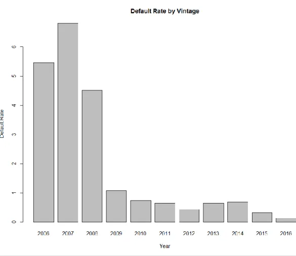
Fannie Mae default rates by year of origination
Figure 2.1. Histogram of default rate (measured in percentage) by year of mortgage origination (i.e. the year the mortgage loan was initiated.)
Exploring the mortgages for defaults across the year of origination, figure 2.2 depicts a high level of performance deterioration for loans that originated in 2006 to 2008. In 2007 nearly more than 10% of the loans that originated in that year entered default at
8
some point. A closer look at mortgages that originated in 2006 to 2008 indicated the highest level of reckless lending.
Performance improved drastically through 2009 to 2016. This can be attributed to certain factors. Firstly, as a result of the crisis, regulatory agencies were forced to improve risk appraisal and tighten lending criteria. Secondly, the default is not immediate; it takes a bit of time for a loan to enter into default.
It was also interesting to explore the data for geographical performances. Figure 2.3 gives the geographical performance of the data as related to default rates.
Fannie Mae default rates across states
Figure 2.2. Default rate (measured in percentage) for each state in the United states. We try to examine how each state performed during the crisis.
9
Puerto Rico (PR) with the capital San Juan jumps out with the highest default rates. In fact, about 10% of loans that originated from this city entered default. This is no surprise, as this city had a high level of foreclosures between 2009 and 2016. According to a statement by Professor Ricardo Ramos, published by Associated Press,
‘’In this U.S. territory of 3.4 million people, local courts oversaw foreclosures on nearly 33,000 homes from 2009 to 2016, according to government statistics. A record 5,424 homes were foreclosed last year, up to 130 percent from nearly a decade ago, when the government first began tracking those numbers. However, the actual number of foreclosures is much higher because the statistics do not include an estimated 20,000 loans in default or close to default that local banks have sold to companies outside Puerto Rico since 2009, Ramos said. Those cases are largely handled in federal court and no one compiles statistics.’’
The high level of default in Puerto Rico was driven by risky bad loans and a weakened economy. Other states with relatively high default rates include Florida (FL), Louisiana (LA), New Jersey (NJ) and New York (NY). This is a clear pointer that states might be an important variable to be considered in our modelling.
Some other variables explored based on prior knowledge include Credit score, loan-to-value ratio (LTV), First-Time-Home-Buyer indicator (FTHB), occupancy status, and loan purpose.
10
Figure 2.3. A graph depicting inverse relationship between credit score and default rate (calculated in percentage).
11
Figure 2.5. Percentage of default, paying and prepaid loans for each category of first-time-home-.buyer.
Figure 2.6. Percentage of default, paying and prepaid loans for each category of occupancy status. (OCC_STAT implies occupancy status described in section 2.2).
12
Figure 2.7. Percentage of default, paying and prepaid loans for each category of loan purpose. Loan purpose specifies if a mortgage loan is purchased, refinanced or cashed-out, each of these categories is denoted by P, R and C respectively (and U, as not specified).
Figure 2.4 is a graph of default rate against credit score. As expected, the graph depicts inverse relationship, the higher the credit score the lower the default rate and vice versa. It is clear that credit score is used to mitigate against default. Borrowers with high credit score are less likely to default. The highest credit score is 850 with default rate less than 1% while the lowest credit score is 550 with default rate of about 19%. In figure 2.5 default rate is plotted against loan-to-value ratio, it is observed that a high LTV ratio corresponds to a high default rate. Figures 2.6, 2.7 and 2.8 examine the impacts of First time home buyer, occupancy status and loan purpose on default rate.
2.2 Variable Description
As previously stated, the variables selected as predictors from the Fannie Mae dataset can be classified into categorical and noncategorical variables. The categorical variables are the First Time Home-buyer Indicator (Yes, No, or Unknown), the Loan
13
Purpose indicator (Primary, Refinance, or Cash-out Refinance), the Credit Score, Occupancy indicator (Owner-Occupied or Investment home), and State indicators for all 50 states. The First Time Home-Buyer Indicator (hereafter FTHB) is a variable that indicates if a borrower or co-borrower is a first-time home buyer or not. According to the description by data supplier (Fannie Mae) we regard an individual as a first time buyer or first time home buyer(FTHB) if he falls into any of these categories: 1) He or she is purchasing the property directly; 2) he or she has maintained no ownership interest solely or jointly in a residential property during the three year period that precedes the property purchase; 3) he or she will directly occupy the property. Similarly, we also categorize as first-time home buyers single parent or displaced homemaker if he or she maintained no sole or joint interest in a residential property during the three-year period that precedes the property purchase.
Loan purpose specifies if a mortgage loan is purchased, refinanced or cashed-out, each of these categories is denoted by P, R and C respectively (and U, as not specified, in some cases). Occupancy status explains how the borrower had specified to use the property at the time of origination. This has been classified as a principal residence (P), second home (s) and investment property (I). Lastly, we have state indicator for 50 states.
For the non-categorical variables, we have Loan Age in months, Unemployment rate, Year of origination of the loan, Credit score, an Original interest rate of the mortgage, Rent ratio, Loan to value ratio, and Debt to Income ratio. Loan age measures the length of months from origination till the loan accrues interest. This is calculated as monthly reporting period - first payment date +1. Credit scores are calculated using proprietary statistical model built specifically for credit and loan data, the credit score used in this dataset is the FICO credit score which was developed by Fair Isaac Corporation. These scores have values ranging from 300 to 850, with 300 denoting weakest score and 850 as the strongest score. Original interest rate captures interest rate on the mortgage at the point of acquisition while debt to income ratio (hereafter referred to as DTI) is measured by taking the ratio of the borrower’s total monthly obligations (including housing expense) to his or her stable monthly income. For our dataset, this variable is measured
14
in percentage and takes values between 1% and 64%. Originating year shows the year the mortgage was acquired. The unemployment rate was measured monthly across the 50 states and linked to the Fannie Mae dataset by state and month. Similarly, rent ratio which was available in 2 sets, for 2010 to 2016 by States and 2006 to 2009 was by monthly average, again this was linked to loan data by month of origin of the loan and by state.
For the output variable, we created three classes namely default (loans that missed monthly repayments for 3 consecutive months), prepaid (loans that were fully paid before or after the expiration of the mortgage) and paying (loans that are still active). We calculated default using current loan delinquency status given in the data. Delinquency status measures a number of days the borrower is delinquent (i.e. couldn’t meet up with monthly obligations) as specified by the governing documents. In the data, status 0 implies current or less than 30 days, status 1 implies greater than 30 days but less than 60 days, status 2 implies greater than 60 days but less than 90 days while status 3 refers to delinquency for days between 90 and 119. We calculated maximum delinquency status for each loan and then specify the output variable as follows: if the maximum delinquency status is greater than 3 (i.e. loan is of delinquency status 3 and above) or zero balance code is greater than 9 (zero balance code is used to indicate why the loan balance was reduced to zero, 09 indicates deed in lieu loans) we classify such loan as default. If the zero-balance code is 01 (01 indicates prepaid or matured loans) we classify such loans as prepaid, the rest of the loans we classify as paying.
15
Chapter Three
3.1 Logistic Regressions
Logistic regression model was developed first in 1958 by David Cox. It is a statistical method utilized in machine learning to assess the relationship between a dependent categorical variable (output) and one or more independent variables (predictors) by employing a logistic function to evaluate the probabilities. Logistic regression can be binary (output variable has two classes), multinomial (output variable has more than two classes) or ordinal.
The logistic function is given by the formula below:
𝑓(𝑥) = 1
1 + 𝑒−(𝛽0+𝛽1𝑥) . (1)
In the above equation f(x) represents the probability of output variable equaling a ‘’ case ‘’, 𝛽0 is interpreted as the linear regression intercept and 𝛽1 is the multiplication of the
regression coefficient by some value of the independent variable. Equation (1) is a positive monotonic modification of linear regression model which enables us to retain the linear pattern of the model as well as ensuring outputs takes values between zero and one. The relationship between logistic models and linear regression can be better expressed by the inverse logistic (also known as logit or log-odds) function given by equation (2) below: 𝑓(𝑥) 1 − 𝑓(𝑥) = 𝑒 (𝛽0+𝛽1𝑥) . (2)
We can see that equation (2) is a simple transformation of linear regression equation i.e.
H(f(x)) = ln [ 𝑓(𝑥)
16
Where H is the log odds which are the odds of the output variable equaling a case and ranges between minus infinity and positive infinity. Similarly, equations (1) and (2) can be represented in terms of multiple independent variables by expressing the exponential function to capture the multiple variables.
Since the performance status of a mortgage loan (default, paying and prepaid) is a qualitative data represented by using categorical variables, clearly, a logistic model is suitable to model this status. We now proceed to implement simple and multinomial multi-class logistic regressions on our mortgage loan dataset.
3.1.1 Simple Logistic Regression
In the simple logistic regression model, the output variable has two classes (e.g. 0 or 1). By definition, the simple logistic regression has output variable with at most two classes (i.e. binary variable which takes values 0 or 1). In our application, value 1 represents the probability of loan status being default and 0 is the probability of loan status equaling paying. This information can be represented in form of a logistic equation as shown below:
𝑃 (𝑙𝑜𝑎𝑛 𝑠𝑡𝑎𝑡𝑢𝑠 = 𝑑𝑒𝑓𝑎𝑢𝑙𝑡 𝑜𝑟 1) = 1
1 +𝑒−(𝛽0+𝛽1𝑥+⋯..+𝛽𝑘𝑥𝑘) . (4a)
where k is the number of independent variables. Here the logit (or odds) is given as
𝑓(𝑥) 1 − 𝑓(𝑥)= 𝑒
(𝛽0+𝛽1𝑥+⋯..+𝛽𝑘𝑥𝑘) . (4b)
where f(x) is the probability of a mortgage loan being default. The logit gives the impact of predictors on the probability of default. Using equation (4a) along with the values of the independent variables we compute the predicted probability of default. This probability gives the basis for our classification, we specify that mortgages with predicted probability lower than 0.6 as ‘’paying’’ and those above 0.6 as ‘’ default’’.
17
The model was constructed using the ‘glm’ function of the ‘caTools’ package in R. Tables 3.1 and 3.2 show the output of the model and the confusion matrix respectively
SIMPLE LOGISTIC MODEL RESULTS
Coefficients:
Estimate Std. Error z value Pr(>|z|)
(Intercept) -2.970e+03 4.001e+01 -74.226 < 2e-16 ***
Loan.Age 1.020e-01 1.616e-03 63.095 < 2e-16 ***
Unemployment_Rate 1.441e-01 5.234e-03 27.536 < 2e-16 ***
Year 1.473e+00 1.984e-02 74.270 < 2e-16 ***
CSCORE_B 1.319e-02 1.577e-04 83.656 < 2e-16 ***
ORIG_RT.x -5.636e-01 1.711e-02 -32.936 < 2e-16 ***
Rent_ratio 7.183e-02 3.026e-03 23.733 < 2e-16 ***
OCLTV -2.885e-02 6.382e-04 -45.202 < 2e-16 ***
DTI -3.190e-02 7.461e-04 -42.748 < 2e-16 ***
OCC_STATP -7.487e-01 3.148e-02 -23.783 < 2e-16 ***
OCC_STATS -1.373e-01 5.153e-02 -2.664 0.007732 **
PURPOSEP 5.360e-01 2.288e-02 23.431 < 2e-16 ***
PURPOSER 1.615e-01 2.108e-02 7.660 1.87e-14 ***
PURPOSEU 6.863e+00 4.978e+01 0.138 0.890352
18
FTHB_FLGY 8.109e-02 2.617e-02 3.098 0.001949 **
STATEAL -7.917e-01 2.451e-01 -3.229 0.001240 **
STATEAR -7.679e-01 2.571e-01 -2.987 0.002821 **
STATEAZ -1.399e+00 2.403e-01 -5.824 5.73e-09 ***
STATECA -1.629e+00 2.371e-01 -6.871 6.39e-12 ***
STATECO -8.551e-01 2.449e-01 -3.491 0.000480 ***
STATECT -1.476e+00 2.437e-01 -6.055 1.41e-09 ***
STATEDC -1.281e+00 2.825e-01 -4.536 5.74e-06 ***
STATEDE -1.303e+00 2.633e-01 -4.950 7.43e-07 ***
STATEFL -1.468e+00 2.374e-01 -6.182 6.34e-10 ***
STATEGA -1.139e+00 2.403e-01 -4.740 2.14e-06 ***
STATEGU 2.884e-01 6.957e-01 0.415 0.678492
STATEHI -1.526e+00 2.551e-01 -5.984 2.18e-09 ***
STATEIA -7.939e-01 2.521e-01 -3.150 0.001635 **
STATEID -1.080e+00 2.549e-01 -4.237 2.27e-05 ***
STATEIL -1.380e+00 2.384e-01 -5.786 7.22e-09 ***
STATEIN -8.212e-01 2.441e-01 -3.364 0.000769 ***
STATEKS -8.893e-01 2.607e-01 -3.411 0.000648 ***
STATEKY -8.835e-01 2.527e-01 -3.496 0.000472 ***
19
STATEMA -1.518e+00 2.411e-01 -6.296 3.05e-10 ***
STATEMD -1.480e+00 2.404e-01 -6.154 7.56e-10 ***
STATEME -1.182e+00 2.666e-01 -4.434 9.23e-06 ***
STATEMI -8.243e-01 2.414e-01 -3.415 0.000637 ***
STATEMN -9.791e-01 2.435e-01 -4.021 5.80e-05 ***
STATEMO -8.329e-01 2.444e-01 -3.408 0.000653 ***
STATEMS -9.403e-01 2.533e-01 -3.712 0.000206 ***
STATEMT -1.230e+00 2.673e-01 -4.600 4.23e-06 ***
STATENC -1.030e+00 2.411e-01 -4.272 1.94e-05 ***
STATEND -1.124e+00 3.137e-01 -3.583 0.000339 ***
STATENE -6.178e-01 2.689e-01 -2.298 0.021571 *
STATENH -1.066e+00 2.616e-01 -4.076 4.59e-05 ***
STATENJ -1.809e+00 2.389e-01 -7.574 3.61e-14 ***
STATENM -9.167e-01 2.535e-01 -3.616 0.000300 ***
STATENV -1.785e+00 2.448e-01 -7.291 3.08e-13 ***
STATENY -1.499e+00 2.380e-01 -6.297 3.04e-10 ***
STATEOH -7.580e-01 2.409e-01 -3.147 0.001652 **
STATEOK -7.014e-01 2.512e-01 -2.792 0.005237 **
STATEOR -1.184e+00 2.443e-01 -4.847 1.25e-06 ***
20
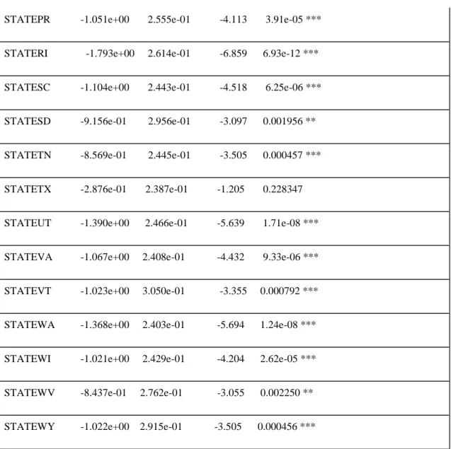
STATEPR -1.051e+00 2.555e-01 -4.113 3.91e-05 ***
STATERI -1.793e+00 2.614e-01 -6.859 6.93e-12 ***
STATESC -1.104e+00 2.443e-01 -4.518 6.25e-06 ***
STATESD -9.156e-01 2.956e-01 -3.097 0.001956 **
STATETN -8.569e-01 2.445e-01 -3.505 0.000457 ***
STATETX -2.876e-01 2.387e-01 -1.205 0.228347
STATEUT -1.390e+00 2.466e-01 -5.639 1.71e-08 ***
STATEVA -1.067e+00 2.408e-01 -4.432 9.33e-06 ***
STATEVT -1.023e+00 3.050e-01 -3.355 0.000792 ***
STATEWA -1.368e+00 2.403e-01 -5.694 1.24e-08 ***
STATEWI -1.021e+00 2.429e-01 -4.204 2.62e-05 ***
STATEWV -8.437e-01 2.762e-01 -3.055 0.002250 **
STATEWY -1.022e+00 2.915e-01 -3.505 0.000456 ***
Table 3.1. Simple Logistic Regression - Default vs. Paying summary statistics
Signif. codes: 0 ‘***’ 0.001 ‘**’ 0.01 ‘*’ 0.05 ‘.’ 0.1 ‘ ’ 1
(Dispersion parameter for binomial family taken to be 1)
Null deviance: 275740 on 499999 degrees of freedom Residual deviance: 127058 on 499932 degrees of freedom AIC: 127194
21
In table 3.1, the estimates represent the coefficient of each variable (i.e. 𝛽𝑖′𝑠) in the logistic regression. The z-value is computed by dividing the estimates or coefficients by its standard error. The z´values (also known as z-statistics) are the results of standardizing the logistic regression estimates while determining whether or not the individual Xi’s variables are related to the output (loan status = default). These values
are calculated as the test statistics for the hypothesis test that the true regression estimate is statistically and significantly close to zero. The p values (Pr(>|z|)) give the decision on whether or not a variable is important in predicting the default class. The smaller the p value the more confident we are about the existence of a strong relationship between the predictor and the output variable. The significance levels are denoted by ‘***’,’**’.’*’,’.’ and ‘ ‘ with ‘***’ as the most significant as 0% level and ‘ ‘ as non-significant. At 1% significant level all variables except two states (Texas and Guam i.e. STATETX and ‘STATEGU’) and first time home buyer indicator category U (non-specified) were statistically significant. The null deviance represents the deviance for the intercept. To compare the performance of our model with that of the null hypothesis (i.e. model with only one variable which is the intercept) we simply compute the difference between the null deviance and the residual deviance. The bigger the difference the better our model is and we can sure reject the null hypothesis that only the intercept is needed for classification and accept the alternative hypothesis that the variables are significant. From table 3.1, the difference between the null deviance and the residual deviance is 148,682 so it is safe to accept the alternative hypothesis.
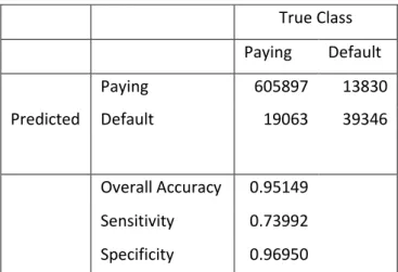
True Class Paying Default Paying 605897 13830 Predicted Default 19063 39346 Overall Accuracy 0.95149 Sensitivity 0.73992 Specificity 0.96950
22
Table 3.2 shows the confusion matrix of the simple logistic model. A random sample of one million seven hundred thousand were chosen from the entire data set. About 60% of the randomly selected subset was used to train the model while the remaining 40% was used as a test set with overall accuracy of the model as 95%.
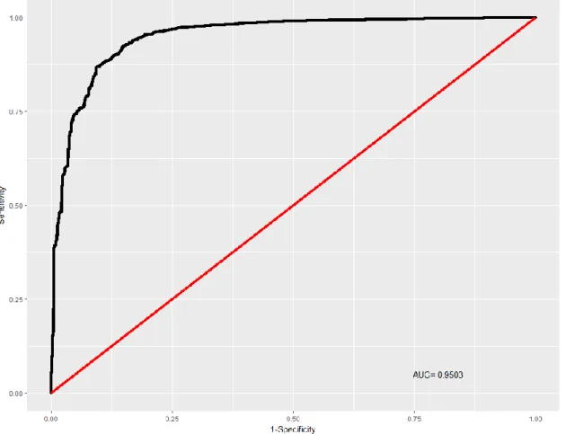
Figure.3.1. ROC Curve - Simple Logistic Regression
Figure 3.1 is a graphical representation of the tradeoff between the percentage of true positives and false positives for every possible cut-off. This is known as the Receiver Operating Characteristic (ROC) curve. The accuracy of the model is measured by the area under the ROC curve. The closer the AUC value is to 1 the more statistically
23
accurate the model is. The simple logistic regression has shown high level of accuracy with AUC = 0.9503.
3.1.2 Multi-class Multinomial Logistic Regression
In multi-class multinomial logistic regression, the output variable has more than two classes. This model is based on the following assumptions: each independent variable has a single value for each case, collinearity is low, and that observed feature has a linear relationship (see http://data.princeton.edu/wws509/notes/c6s2.html). One simple way to implement multinomial logistic model is to first implement i-1 binary logistic models where i is the possible number of outcomes. We take any of these possible outcomes as ‘’pivot’’ or ‘’ base’’ and then perform regression iterations on the remaining i-1 outcomes separately. This can be expressed mathematically as follows: If we take the ith outcome as base (last outcome) we have,
𝑙𝑛 [𝑃(𝑌𝑘= 1)
𝑃(𝑌𝑘= 𝑖)] = 𝛽1𝑋𝑘 . (5)
We can further equation (5) below:
𝑙𝑛 [𝑃(𝑌𝑘= 𝑖 −1)
𝑃(𝑌𝑘= 𝑖) ] = 𝛽𝑖−1𝑋𝑘. (6)
We can therefore determine the probabilities by taking the exponential of equation (6) and keeping in mind that all i probabilities must sum to one. We then have,
𝑃(𝑌𝑘 = 𝑖 − 1) =
𝑒(𝛽𝑖−1𝑋𝑘)
24
Financial institutions also consider the risk of ‘prepay’ (loss of income) on loans, so it is necessary to create the ‘’ prepaid ‘’ class and then use the multi-class multinomial model to predict the three possible outcomes namely: default, prepaid and paying. In our application, we take the default group as the pivot and then model estimates for paying and prepaid mortgages. Therefore, the odds of a loan falling in group i as against the default group (base) can be expressed below:
𝑙𝑛 [ 𝑃(𝑙𝑜𝑎𝑛 𝑠𝑡𝑎𝑡𝑢𝑠 = 𝑖)
𝑃(𝑙𝑜𝑎𝑛 𝑠𝑡𝑎𝑡𝑢𝑠 = 𝑑𝑒𝑓𝑎𝑢𝑙𝑡)] = 𝛽0 𝑖 + 𝛽
1𝑖𝑋𝑘+ ⋯ + 𝛽𝑘𝑖𝑋𝑘, (8)
where group i = paying or prepaid and the 𝛽′𝑠 are estimates measuring the effect of a variable on a mortgage falling in group i as against the pivot’s (or base) group. Using equation 8 we estimate the probability that a loan will fall into prepaid or paying by the equation below: 𝑃(𝑙𝑜𝑎𝑛 𝑠𝑡𝑎𝑡𝑢𝑠 = 𝑖) = 𝑒(𝛽0𝑖 +𝛽1𝑖 𝑋𝑘+⋯+𝛽𝑘𝑖 𝑋𝑘) ∑ 𝑒(𝛽0𝑖 +𝛽1𝑖 𝑋𝑘+⋯+𝛽𝑘𝑖 𝑋𝑘) 𝑖 . (9)
The choice of the base group will determine the value of the coefficient estimate but the predicted probability will remain the same regardless of the base group choice. A mortgage is therefore assigned to the class of the highest predicted probability.
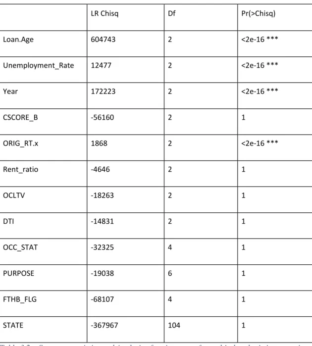
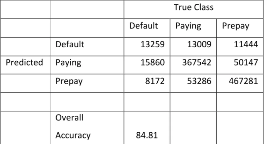
The multinomial logistic regression model was created using nnet (neural network) package in R using 2.5 million rows of randomly selected dataset with 60% (1.5 million rows of dataset) of the data set used to train the model. The model converged after 70 iterations. The model was tested on a sample of 1 million test data to predict the relative probability of each class. The overall accuracy of the model is 74.08% when all the initial twelve variables were considered. The accuracy, however, increased to 84.81% when 5 variables were dropped using backward elimination (DTI, OCC_STAT, PURPOSE, FTHB_FLG , STATE) as shown in tables 3.3b and 3.4.
25
Analysis of Deviance Table (Type II tests) Response: Loan_Status LR Chisq Df Pr(>Chisq) Loan.Age 604743 2 <2e-16 *** Unemployment_Rate 12477 2 <2e-16 *** Year 172223 2 <2e-16 *** CSCORE_B -56160 2 1 ORIG_RT.x 1868 2 <2e-16 *** Rent_ratio -4646 2 1 OCLTV -18263 2 1 DTI -14831 2 1 OCC_STAT -32325 4 1 PURPOSE -19038 6 1 FTHB_FLG -68107 4 1 STATE -367967 104 1
Table 3.2a. Summary statistics and Analysis of variance test for multi-class logistic regression
26
Multinomial Logistic Regression
True Class
Default Paying Prepay Default 13333 19452 20725 Predicted Paying 15378 304818 85440 Prepay 8409 109811 422634
Overall
Accuracy 74.08
Table 3.3b. Confusion Matrix for Multinomial Logit with 12 variables
True Class
Default Paying Prepay Default 13259 13009 11444 Predicted Paying 15860 367542 50147 Prepay 8172 53286 467281
Overall
Accuracy 84.81
Table 3.4. Confusion matrix for Multinomial Logit with 7 variables (5 variables were dropped)
Table 3.3a gives the performance of each variable in the model. The most significant variables in the model were loan age, unemployment rate, original rate and year of origination with p values less than 2e-16. The model validation was done with the likelihood ratio test for Chi-square (see column LR Chisq in table 3.3a ) at various degree of freedoms ( DF ). Other variables with higher p values suggest that the model give almost same accuracy without these variables. This implies that dropping these variables may likely not affect the overall performance of our model.
27
3.2 Naive Bayes Classifier
The study of Naive Bayes is dated back to the 1950s. It is sometimes referred to as simple Bayes and independence Bayes. Naive Bayes classifier is from a group of probabilistic classifiers derived by using the Bayes theorem and holds the assumption that if the class is known, the attributes of a sample are independent. Generally speaking, Naive Bayes classifier is a conditional probabilistic model that includes a decision rule, one of such rules is the MAP rule or maximum a posteriori rule.
If we imagine a supervised learning task where the aim is to approximate a target function P(X/Y). This can be represented in Bayes form as
𝑃(𝑌 = 𝑦𝑖|𝑥1, 𝑥2, … , 𝑥𝑗) = 𝑃(𝑋 = 𝑥1,𝑥2,…,𝑥𝑗| 𝑌= 𝑦𝑗)∗𝑃(𝑌 =𝑦𝑖 )
∑ 𝑃(𝑋 = 𝑥𝑗1 1,𝑥2,…,𝑥𝑗| 𝑌= 𝑦𝑗)∗𝑃(𝑌 =𝑦𝑖 )
(10)
Since our main interest is the result of the classification task, we then assign the instance Y the class with the highest probability.
𝑌 ← 𝑎𝑟𝑔 𝑚𝑎𝑥 𝑃( 𝑌 = 𝑦𝑖) ∏ 𝑃(𝑥𝑗1 𝑖|𝑌 = 𝑦𝑖) (11)
Applying the above to our dataset, conditional probabilities were calculated for all categorical variables while means and standard deviation were computed for numeric variables. The model was constructed using the ‘e1071’ package in R. One million sample sizes were randomly selected with 50% as training set and 50% as a test set. Table 3.5 shows the performance result of the model.
28
True Class
Default Paying Prepay
Default 13323 2720 2329
Predicted Paying 9102 184878 23400 Prepay 22534 86215 155499
Overall
Accuracy 70.74%
Table 3.5. Confusion for Matrix Naive Bayes
Using the confusion matrix function in R, we generate the overall statistics of the model as shown below:
Accuracy : 0.7074 95% CI : (0.7061, 0.7087)
No Information Rate : 0.5476 P-Value [Acc > NIR] : < 2.2e-16
Kappa : 0.484 Mcnemar's Test P-Value : < 2.2e-16 Statistics by Class:
Class: Default Class: Paying Class: Prepay Sensitivity 0.29634 0.6752 0.8580 Specificity 0.98890 0.8563 0.6589 Pos Pred Value 0.72518 0.8505 0.5885 Neg Pred Value 0.93431 0.6853 0.8909 Prevalence 0.08992 0.5476 0.3625 Detection Rate 0.02665 0.3698 0.3110 Detection Prevalence 0.03674 0.4348 0.5285 Balanced Accuracy 0.64262 0.7658 0.7584
29
The P value and Mcnemar's Test P-Value shows the variables were statistically significant although the overall accuracy of the model was lower compared to the logistic models. The kappa statistic measures how closely the instances classified by the naive Bayes model match the original data class. The kappa value of 0.484 shows our model performed moderately. The positive predicted value (Pos Pred Value) was the lowest for the prepaid class (merely 58.85%) and highest for the default class
30
Chapter Four
4.1 Random Forest Model
Random forest model is an ensemble machine learning method for performing classification or regression tasks This is achieved by constructing several decision trees and then giving as output the class that is the most occurring (mode) of the classes for classification and mean prediction for regression tasks. In this section we focus on random forest for classification tasks. Random forest models make use of random selection of features in splitting the decision trees, hence the classifier built from this model is made up of a set of tree-structured classifiers. We can represent the random forest model by equation (12) below:
𝑆𝑝𝑎𝑐𝑒 = {𝐹(𝑋, 𝛼𝑖); 𝑖 = 1,2,3,4, . . . , 𝑛𝑜𝑠 𝑜𝑓 𝑡𝑟𝑒𝑒𝑠} (12)
In equation (12), 𝛼𝑖 represents the number of independent and identically distributed
random vectors in a way that every tree has a vote for the most popular class. To build the algorithm for this model, we pick at random k data points from the training set and build a decision tree associated to these k data points. Next, we choose the number of trees (ntrees) we desire to build and then repeat the previous steps. For a new data point, we make our ‘ ntrees’ predict the category to which the data point belongs and then assign the new data point to the class that wins majority votes. We start with one tree and then proceed to build more trees based on the subset of data.
The random forest has a major advantage that it can be used to judge variable importance by ranking the performance of each variable. The model achieves this by estimating the predictive value of variables and then scrambling the variables to examine how much the performance of the model drops.
31
In applying the random forest model to our dataset, random sample of one million observations were used to create a random forest model using all the twelve predictors. Exactly 60% of the data was used as training set while the remaining 40% was used as test set using R package “randomForest”. This package also provided the variable importance/ ranking shown in figure 4.1, variable importance of the model tells which variable has highest impact in making the prediction using 2 metrics namely Mean decrease in accuracy (MDA) and Mean decrease in Gini. Mean decrease in accuracy is percentage or proportion of incorrectly classified observations when a particular variable is excluded from the model. The MDA is computed for each tree by permuting the out-of-bag (OOB) data and then recording the prediction error. The error difference for each successive permutation is then averaged and normalized by the standard deviation. On the other hand, the mean decrease in gini measures the average increase of purity achieved by the splits of a variable. If such variable is important in the model it will achieve a split of mixed classes nodes into single class nodes.
32
RANDOM FOREST
ntree formula0 formula1 formula2 formula3 formula4 formula5 formula6 formula7 formula8 formula9
10 0.949 0.953645 0.95374 0.953633 0.952528 0.953763 0.954635 0.95335 0.92575 0.937253 20 0.952543 0.954593 0.95584 0.955373 0.95422 0.95492 0.955118 0.953768 0.934913 0.940028 30 0.95312 0.95569 0.956413 0.955758 0.954903 0.955235 0.95541 0.954043 0.934383 0.939333 40 0.953885 0.955878 0.95622 0.956015 0.954905 0.955578 0.95541 0.954095 0.93602 0.941858 50 0.954158 0.955665 0.95659 0.956003 0.955078 0.955503 0.955318 0.954165 0.935023 0.941095 60 0.954448 0.955958 0.956688 0.9562 0.95515 0.95548 0.955513 0.954328 0.9354 0.94106 70 0.954478 0.956185 0.956645 0.95624 0.955175 0.955863 0.955715 0.95422 0.93407 0.941063 80 0.954353 0.956205 0.95653 0.956185 0.955125 0.955595 0.955503 0.95415 0.935788 0.942295 90 0.954878 0.956163 0.956593 0.95641 0.955208 0.955603 0.955568 0.954248 0.935575 0.940908 100 0.954573 0.956245 0.956575 0.95635 0.955275 0.955758 0.9556 0.954363 0.935958 0.94218 110 0.955008 0.95617 0.956708 0.956465 0.95528 0.955735 0.955713 0.95438 0.93584 0.94163 120 0.954898 0.956313 0.9566 0.956425 0.955488 0.955648 0.95562 0.954335 0.933968 0.942425 130 0.954903 0.95628 0.956745 0.95649 0.955348 0.955715 0.95575 0.95431 0.936173 0.94127 140 0.954958 0.956253 0.95678 0.956375 0.955405 0.955658 0.955713 0.954313 0.934788 0.94249 150 0.955058 0.956368 0.956728 0.956533 0.955453 0.955725 0.955565 0.95435 0.936423 0.941585
Table 4.1. Accuracies of Random Forest model for 10 to 150 trees and 10 different permutation of variables.
33
Figure 4.1. Random Forest variable importance/ ranking using mean decrease in accuracy and mean decrease in gini.
From the variable importance chart, Loan Age has highest impact using both metrics and State has least impact in making prediction using the mean decrease accuracy metric while first-time-home-buyer indicator has the least impact using the mean decrease in gini metric. One hundred and fifty different random forest models were created using fifteen different number of trees from (10, 20,…..150) and 10 different formulas. For example, we see that over 120,000 observations will be misclassified if we drop the variable ‘Loan age’ from our model while dropping first-time-homebuyer will result in no changes in the accuracy of our model. We permuted the variables by removing the least important variable from the equation at each step. In the accuracy table (shown in table 4.1) ‘formula0’ represents the inclusion of all twelve variables, ‘’formula1’’ consist of 11 variables (state variable was dropped) and so on. Accuracies of these models are presented in table 4.1. The highest accuracy of the model is 0.95678 produced at formula2 which consist of 10 variables (First-time-homebuyer and state variables were dropped) at 140 trees. Confusion matrix and overall statistics of the same are presented below.
34
Accuracy : 0.9568
95% CI : (0.9557, 0.9569) No Information Rate : 0.5283 P-Value [Acc > NIR] : < 2.2e-16
Kappa : 0.9173 Mcnemar's Test P-Value : < 2.2e-16 Statistics by Class:
Class: Default Class: Paying Class: Prepay Sensitivity 0.53570 0.9773 0.9686 Specificity 0.98996 0.9501 0.9877 Pos Pred Value 0.67298 0.9377 0.9888 Neg Pred Value 0.98223 0.9819 0.9656 Prevalence 0.03715 0.4346 0.5283 Detection Rate 0.01990 0.4247 0.5117 Detection Prevalence 0.02957 0.4529 0.5175 Balanced Accuracy 0.76283 0.9637 0.9782
True Class
Default Paying Prepay
Default 7960 3497 321
Predicted Paying 5031 169877 6260
Prepay 1868 453 204683
Overall
Accuracy 95.68%
35
From the model statistics, Kappa’s value of 0.9173 suggests that our model performs very well while the p value < 2.2e-16 indicates that the selected variables were statistically significant at 1% significance level. In predicting the paying and prepaid class the model performed extremely well with sensitivity and specificity for both classes exceeding 90%. However, the model performed moderately in predicting the default class with sensitivity just above 50%. Overall, the model performed very well with accuracy above 95%.
4.2 KNN Model
The K Nearest Neighbor classifier (also known as KNN) is an example of a non-parametric statistical model, hence it makes no explicit assumptions about the form and the distribution of the parameters. KNN is a distance based algorithm, taking majority vote between the k closest observations. Distance metrics employed in KNN model includes for example Euclidean, Manhattan, Chebyshev and Hamming distance. In this work we apply only the Euclidean distance measure. The KNN algorithm can be summarized as follows: given a positive integer K, a distance metric d and an unknown observation x, the model performs the steps below:
1) First it goes through the entire training set calculating the distance d between x and each data point in our training set. Taking K points closest to x as W and such that K is always an odd number to prevent a tie. 2) Next, we compute the proportion of points in W associated with a given
class label. This is called the conditional probability of each class and is given by equation (13) below:
𝑃(𝑦 = 𝑖|𝑋 = 𝑥) = 1
𝐾∑ 𝐼(𝑦
(𝑗) = 𝑖) 𝑊
𝑗∈𝑊 (13)
In equation (13) I is an indication function which evaluates to 1 when x is true and zero when x is false. Lastly, we classify x to the class with the highest probability.
36
The choice of K is of great importance. This is because in KNN, K is a hyperparameter that controls the shape of the decision boundary and must be properly set in order to attain the best possible fit for the data set. Small K will restrain the prediction region and thus lead to high variance with low bias. Conversely, a higher choice of K accommodates more voters in the prediction region thus leading to a smoother decision boundary which implies lower variance but with increased bias. It should be noted that KNN training phase comes with both memory cost and computational cost. Memory cost is due to the fact that we have to store a huge data set because the algorithm simply memorizes the training observations which is used as ‘’ experience or knowledge ‘’ for the classification phase. The implication of this is that the algorithm only uses the training observations to give out predictions when a query is passed into our database. Since predicting the class of a single observation requires going through the entire data set, computational cost is therefore a factor to be considered.
In applying the KNN classifier to our data set, a randomized set of 120,000 data points was selected out of which 80,000 observations was used as training set and 40,000 observations as test data. 50 different KNN model were created with different K values varying from 1 to 50 and accuracy of each model was tested by making prediction on the test data. A plot of these accuracies against k values was obtained (See figure 4.2).
37
True Class
Default Paying Prepay
Default 828 355 184
Predicted Paying 438 16654 4908
Prepay 223 638 15772
Overall
Accuracy 0.83135
Table 4.1. Confusion matrix K- Nearest Neighbors with K = 15
From figure 4.2 we can see that the highest accuracy was achieved at K = 15 with accuracy of approximately 83%. K values higher than 15 did not yield increase in accuracy. The lowest accuracy occurred at K = 3 with accuracy of less than 40%. A careful look at figure 4.2 suggests an interesting situation whereby at smaller values of K, odd K values produced lesser accuracies than even K values (Ordinarily odd values of K should yield higher accuracies) as seen in the case of K = 2 with accuracy of 79% and K = 3 with accuracy of 38%. This scenario is usually as a result of ‘ties’ in the KNN model when allocating votes to different classes. Ties indicate that two or more classes have equal chances or probabilities of predicting the class of a new input. The implication of this is that two or more classes have equal numbers of nearest neighbors (neighbors with equal distances) for the predicted data. Recall that the output variable has 3 classes and as such at K = 3 there’s a high chance of each class having equal votes (for K = 5 tie may occur if 2 classes has equal votes). Ties are natural occurrences in KNN model especially with huge dataset like the one used in this thesis, this is so because the probability of tie occurring increases with the size of data. One way to break ties is to apply a different selection criterion by estimating partial sums of distances to predict each class. Another way is to decrease the size of K by 1 until the tie
38
is eventually solved. However, the R software used in this thesis break ties randomly. Table 4.3 shows the confusion matrix of the K-NN model at K = 15 with overall accuracy of 83%. The model performed very well in predicting the ‘paying’ and ‘prepaid ’classes with positive predicted values of 76% and 94% respectively. However, the model did not perform so well in predicting the default class. The positive predicted value of the default class is 56% which is slightly above average.
Accuracy : 0.8282 95% CI : (0.8244, 0.8319)
No Information Rate : 0.5279 P-Value [Acc > NIR] : < 2.2e-16
Kappa : 0.6797
Mcnemar's Test P-Value : < 2.2e-16
Statistics by Class:
Class: Default Class: Paying Class: Prepay Sensitivity 0.49573 0.9328 0.7637
Specificity 0.98611 0.7647 0.9451
Pos Pred Value 0.56529 0.7547 0.9396
Neg Pred Value 0.98171 0.9362 0.7815
Prevalence 0.03515 0.4370 0.5279
Detection Rate 0.01742 0.4076 0.4032
Detection Prevalence 0.03083 0.5401 0.4291
39
4.3 Survival Analysis and Cox Proportional Hazard Model
4.3.1 Survival Analysis
Survival analysis is a statistical approach of estimating the expected time until an event (the event could be more than one) happens. Taking into consideration the dependence of observations and applying the mortgage contract as a unit of measurement as against the contract year, survival model gives the probability distribution for the length of time until a mortgage falls into any of the 3 classes (defaults, paying and prepaid). The relationship between the covariates and the survival function can be expressed in terms of two models: proportional hazard models and accelerated life models. This relationship can be expressed mathematically as follows:
𝛼𝑖(𝑡, 𝑥) = 𝑙𝑖𝑚 𝛥𝑡→0
𝑃(𝑡 ≤ 𝑇𝑖< 𝑡 + 𝛥𝑡|𝑇𝑖≥𝑡)
𝛥𝑡 = 𝛼𝑖0(𝑡)𝑒
−𝑥′𝜆𝑖 (14)
In equation (14), 𝛼𝑖0(𝑡) is the parameter that describes the distribution of the failure time when the independent variables are equal to zero and T is a discrete random variable suggesting the survival time. At different times, the status of a mortgage could vary. Usually a mortgage life starts at status ‘paying’ and later moves to either ‘fully prepaid’ or ‘default’, but in credit risk context financial institutions are also interested in ''WHEN'' a loan will likely default. For example, a loan that is '' paying'' at the time of data gathering, it is obvious that such loan hasn't defaulted yet but one cannot categorically conclude that such loan will not default since it has not reached the maturity period date yet. Therefore, we can express equation (14) in terms of the relationship between mortgage status, independent variables and length of time as follow:
𝛼(𝑡) = 𝛼0(𝑡)𝑒(𝜆1𝑥1 + 𝜆2𝑥2 +...+𝜆𝑘𝑥𝑘) (15)
where 𝛼(𝑡)is the conditional probability that a mortgage will survive until a time t and not beyond that, t indicates the loan age in months, 𝑥1, 𝑥2,...,𝑥𝑘are the independent variables that determine the risk of mortgage termination, 𝜆1, 𝜆2,...., 𝜆𝑘 are estimates
40
that evaluates the impacts of the independent variables on the hazard rate and 𝛼0(𝑡)represents the hazard baseline. The hazard baseline captures the shape of the
hazard function and the changes in the probability of mortgage termination (i.e. probability of loan entering default or prepaid status) over time. Since mortgage terminates when loan status is either prepay or default, we can therefore establish the existence of two competing risks. Defaults and prepayments are therefore competing risk because a loan that defaults cannot prepay and a loan that prepays cannot default hence it is important to make use of a competing risks hazard model which analyzes the joint choices of prepayment and defaults as well as evaluates the impact of variables on prepayments and defaults.
The first step in performing a survival analysis is to preprocess the data into loan age structure (in months) and then select an indicator (loan status). We then make use of the time parameter to represent the time before a mortgage changes status from paying to either prepay or default. Using a randomly selected loan observation of 100,000 we generate the survival curve using the survival package in R as shown in figure 4.3 below.
41
Figure 4.3 shows the probability of a mortgage surviving pass a certain number of months before changing status. From the graph it can be deduced that it is very unlikely for a loan to survive pass 150 months without changing status, the probability of survival above 130 months is approximately zero. Using the summary function in R, we obtain the median number of survival month as 58 months with probability of survival approximately 0.5. To explore the survival rate of each category separately, we split the data into ‘default’ and ‘prepaid’ and produce a separate graph for each category as shown below.
42
Figure 4.4b. Survival curve for prepay category (probability of loan status changing from paying to prepay)
From both figures 4.4a and 4.4b we see that probability of paying reduces as the number of months increases. This is as expected, as loan age increases one expects that the loan status will change to either prepay or default.
4.3.2 Cox Proportional Hazard Model
The Cox proportional hazard model is a method for estimating and analyzing the impact of several variables on the specific time until an event happens. To determine the relative impact of each variable with the aim of identifying which variable has the highest impact on default rates a Cox Proportional Hazard model (CPH) is very effective for this purpose. This model has two basic assumptions as follow: a) There exist a default rate which can be taken as the ‘BASEline’ or ‘HAZARD’ rate b) the independent variables are proportional to the baseline rate in a multiplicative way. It should be noted that the Cox model is a semi parametric model which implies that it is
43
defined parametric partially. This suggests that the baseline aspect of the model has no parametric form while the covariate part has a functional form, however if we have prior knowledge of the exact form of the baseline we can then replace the hazard baseline (represented by 𝛼0(𝑡) in equation (15)) by a given function.
To build the Cox model on our dataset, we again make use of the survival package in R and employ the ‘coxph’ function using the randomly selected 100,000 loan observations previously generated for the survival curve. The summary of the model is presented below:
Call:
coxph(formula = formula, data = df) n= 100000, number of events= 1167
coef exp(coef) se(coef) z Pr(>|z|) Unemployment_Rate 5.579e-01 1.747e+00 1.717e-01 3.249 0.001158 **
Year 6.758e-01 1.966e+00 1.556e-01 4.344 1.40e-05***
CSCORE_B -1.882e-02 9.814e-01 6.850e-04 -27.473 < 2e-16 ***
ORIG_RT.x 9.341e-02 1.098e+00 8.043e-02 1.161 0.245495
Rent_ratio -5.191e-01 5.950e-01 5.618e-02 -9.240 < 2e-16 ***
44
DTI 3.315e-02 1.034e+00 3.557e-03 9.317 < 2e-16 *** OCC_STATP -1.182e-01 8.885e-01 1.164e-01 -1.015 0.309993
OCC_STATS -6.409e-01 5.268e-01 1.784e-01 -3.593 0.000327***
PURPOSEP -5.148e-01 5.976e-01 8.662e-02 -5.943 2.80e-09 ***
PURPOSER
-3.627e-01 6.958e-01 8.644e-02 -4.196 2.72e-05 ***
FTHB_FLGU -8.907e+00 1.354e-04 7.358e+02 -0.012 0.990341
FTHB_FLGY 3.135e-01 1.368e+00 9.144e-02 3.429 0.000606 ***
Table 4.1. Cox Regression Model equation summary and variable assessment
Signif. codes: 0 ‘***’ 0.001 ‘**’ 0.01 ‘*’ 0.05 ‘.’ 0.1 ‘ ’ 1
exp(coef) exp(-coef) lower .95 upper.95 Unemployment_Rate 1.7470593 0.5724 1.2478 2.4461 Year 1.9656038 0.5087 1.4490 2.6664
CSCORE_B 0.9813576 1.0190 0.9800 0.9827
45 Rent_ratio 0.5950399 1.6806 0.5330 0.6643 OCLTV 1.0166862 0.9836 1.0110 1.0224 DTI 1.0337019 0.9674 1.0265 1.0409 OCC_STATP 0.8885141 1.1255 0.7072 1.1163 OCC_STATS 0.5268356 1.8981 0.3714 0.7473 PURPOSEP 0.5976107 1.6733 0.5043 0.7082 PURPOSER 0.6958244 1.4371 0.5874 0.8243 FTHB_FLGU 0.0001354 7385.2077 0.0000 Inf FTHB_FLGY 1.3682443 0.7309 1.1438 1.6368
Table 4.2. Cox Regression overall model summary
Concordance = 0.812 (se = 0.009 ) R-square = 0.016 (max possible= 0.155 )
Likelihood ratio test = 1605 on 13 degree of freedom (df), p=0 Wald test = 310.8 on 13 degree of freedom (df), p=0 Score (logrank) test = 1793 on 13 df, p=0
Table 4.1 gives the information about the equation of the Cox Regression model and data sample used in the modelling. For example, sample size is given by n = 100,000 and number of attrition as 1167. Just like every other regression model output, the Cox Regression model output has beta coefficient, standard error, z statistics and a p-value. The ‘’ exp(coef) ‘’ are simply the exponentiation of the beta coefficients and the associated standard error is given in the column ‘’ se(coef)’’. The goodness of fit and statistical significance of each variable can be deduced using the z statistics and the corresponding P-value. Z statistics is computed by dividing beta by its standard error. If the corresponding P-value is lesser than 0.05 ( 5%) we can reject the null hypothesis
46
that the beta value is zero at 95% confidence interval. Table 4.2 gives the overall model performance using certain indicators. Concordance measures the proportion in the sample, where the loan observations with the higher survival period has the higher rate/probability predicted by the cox model while R2 examines the variance explained by our model (R2 of 0.16). Using the likelihood ratio test, Wald test and the score
logrank test we reject the null hypothesis that beta is zero since each of these tests has P-value of zero. Judging by the P-values for each variable from table 4.1, all variables except first-time-homebuyer (category U), original rate and occupancy status (category P) were statistically significant.
The interpretation of the categorical variables (LOAN PURPOSE, OCCUPATIONAL STATUS, and FTHB) is quite easy and straightforward, this can be easily achieved by mere looking at the exp(coef) column to observe their respective effect. For example, looking at the variable Purpose, we see that refinanced loans multiplied the default rate by 0.69 as compared to repurchased loans. On the contrary, interpretation of the continuous variables cannot be easily achieved by mere looking at the coefficients. This can be attributed to the fact that each of the variables have different scales. For example, Loan-To-Value ranges from 30 to 100, Credit scores ranges from 600 to 800 while Debt-To-Income ratios are from 20 to 60. To get a better interpretation of this variables we make use of graphs.
47
Figure 4.5. Hazard rate multiplier for continuous variables
In the above graphs (figure 4.5), the base default rate multiplier (note not the default rate itself) is depicted on the y-axis. To understand this better, for instance the mean current LTV of the dataset is 75 with base multiplier as 1. If we consider two loans where the first loan has a current LTV of 75 and the second has a current LTV as 90, the Cox Proportional Hazard model predicts the second model’s default rate as 1.25 times the default rate of the first.
48
All the predictors from the plot behaved as expected, predictors LTV, DTI, Original rate are directly related to the default hazard rate ( and inversely related to prepaid hazard rate) such that if the LTV increases then the chances of default rate (probability of survival ) also increases where as in the case of Credit score it is inversely related to default hazard rate ( and directly related to prepaid hazard rate ) which means higher credit score has lower default risk and lower credit score has higher default risk.