EVALUATION OF DIAGNOSTIC PERFORMANCE USING PARTIAL AREA UNDER THE ROC CURVE
by
Hua Ma
B.S. Sichuan Normal University, Chengdu, China, 2007 M.S. Xiamen University, Xiamen, China, 2010
Submitted to the Graduate Faculty of the Department of Biostatistics
Graduate School of Public Health in partial fulfillment of the requirements for the degree of
Doctor of Philosophy
UNIVERSITY OF PITTSBURGH GRADUATE SCHOOL OF PUBLIC HEALTH
This dissertation was presented by
Hua Ma
It was defended on May 8, 2014 and approved by
Howard E. Rockette, PhD, Professor, Department of Biostatistics Graduate School of Public Health, University of Pittsburgh
Jong-Hyeon Jeong, PhD, Professor, Department of Biostatistics Graduate School of Public Health, University of Pittsburgh
David Gur, ScD, Professor, Department of Radiology School of Medicine, University of Pittsburgh
Chung-Chou Chang, PhD, Associate Professor, Department of Biostatistics Graduate School of Public Health, University of Pittsburgh
Dissertation Director: Andriy Bandos, PhD, Assistant Professor, Department of Biostatistics, Graduate School of Public Health, University of Pittsburgh
Copyright © by Hua Ma 2014
Andriy Bandos, PhD
EVALUATION OF DIAGNOSTIC PERFORMANCE USING PARTIAL AREA UNDER THE ROC CURVE
Hua Ma, PhD
University of Pittsburgh, 2014
ABSTRACT
Evaluation of diagnostic performance is critical in many fields including but not limited to diagnostic medicine. The Receiver Operating Characteristic (ROC) curve is the most widely used methodology for describing the intrinsic performance of diagnostic tests, with the area under the curve (AUC) being the most commonly used summary index of overall performance. The partial area under the ROC curve (pAUC), when focused on the range of practical/clinical relevance, is considered a more relevant summary index than the full AUC. However, several conceptual and analytical difficulties frequently prevent the pAUC from being used. First, in many diagnostic setting the relevant range is difficult to determine objectively. Second, in theory, due to potential use of less information, analysis based on the pAUC could lead to the loss of statistical precision and therefore would require larger sample sizes. Through mathematical derivation, extensive simulation studies and practical examples, this work investigates statistical properties when using the pAUC. First, this work demonstrates that in many practical scenarios inferences based on pAUC could be more powerful than inferences based on the full AUC. Thus, the use of the pAUC may lead to not only more clinically relevant but also more conclusive results in analyses of experimental data. Second, this investigation demonstrates that the advantages of pAUC-based inferences depend on the shape of ROC curves. The conventional binormal model does not always adequately describe scenarios where the pAUC is more
statistically efficient. The bi-gamma family of concave ROC curves is shown to describe practically reasonable scenarios where either pAUC or full AUC could be advantageous. Programs for sample size estimation based on bi-gamma model are then developed. Finally, this work investigates the properties of pAUC-based inferences in scenarios where diagnostic results have substantial ties (or a “mass”) at the lowest diagnostic results. For certain type of the ROC curves the existence of ties could lead to an increase in statistical efficiency. Forcing a diagnostic system to resolve ties could detrimentally affect reliability and conclusiveness of statistical inferences. In conclusion, this work provides investigators with insights into and tools for generating practically relevant conclusions using pAUC. The public health importance of this work stems from the relevance of the ROC analysis at different stages of development and regulatory approval of diagnostic systems in medicine. Enhanced methodology for evaluation of diagnostic accuracy helps in the development of improved diagnostic systems and could accelerate the delivery and clinical adoption of truly beneficial diagnostic technologies and/or clinical practices.
TABLE OF CONTENTS
1.0 INTRODUCTION ... 1
1.1 BACKGROUND ... 1
1.2 OBJECTIVES ... 6
2.0 FACTS RELATED TO THE PRESEARCH ... 9
2.1 FAMILIES OF ROC CURVE, THEIR AUCS AND PAUCS ... 9
2.1.1 BINORMAL ROC CURVES ... 9
2.1.2 POWER-LAW ROC CURVES ... 10
2.1.3 BI-GAMMA ROC CURVES ... 11
2.1.4 STRAIGHT-LINE ROC CURVES ... 14
2.2 ESTIMATION OF ROC CURVES ... 15
2.2.1 PARAMETRIC ESTIMATES OF ROC CURVES ... 15
2.2.2 EMPIRICAL ROC CURVE ... 17
2.3 ESTIMATION OF AUC AND PAUC ... 18
2.3.1 PARAMETRIC ESTIMATES OF AUC AND PAUC... 18
2.3.2 EMPIRICAL ESTIMATES OF AUC AND PAUC ... 19
2.4 ESTIMATION OF VARIANCE OF AUC AND PAUC ... 20
3.0 EVALUATION OF A SINGLE PAUC ... 23
3.1 METHOD ... 24
3.1.1 STANDARDIZED PARTIAL AUC AND ITS PROPERTIES ... 24
3.1.2 VARIANCE OF THE PARAMETRIC ESTIMATE OF SPAUC ... 28
3.2 NUMERICAL STUDY ... 32
3.4 SUMMARY ... 49
4.0 COMPARISON OF TWO CORRELATED PAUCS ... 51
4.1 METHOD ... 52
4.2 NUMERICAL STUDY ... 59
4.3 EXAMPLES ... 75
4.4 SUMMARY ... 77
5.0 PARTIAL AREA UNDER THE ROC CURVE WITH MASS ... 79
5.1 METHOD ... 80
5.2 NUMERICAL STUDY ... 81
5.2.1 EVALUATION OF A SINGLE PAUC ... 83
5.2.2 COMPARISON OF CORRELATED PAUC ... 89
5.3 SUMMARY ... 95
6.0 CONCLUSION AND DISCUSSION ... 97
6.1 EVALUATION OF A SINGLE PAUC ... 98
6.2 COMPARISON OF TWO CORRELATED PAUCS ... 99
6.3 PARTIAL AREA UNDER THE ROC CURVE WITH MASS ... 101
APPENDIX A ... 104
ON USE OF PARTIAL AREA UNDER THE ROC CURVE FOR EVALUATION OF DIAGNOSTIC PERFORMANCE ... 104
APPENDIX B ... 105
ON THE USE OF PARTIAL AREA UNDER THE ROC CURVE FOR COMPARISON OF TWO DIAGNOSTIC TESTS ... 105
R PROGRAM FOR ESTIMATING SAMPLE SIZES FOR BI-GAMMA ROC CURVES IN EVALUATION OF SINGLE PARTIAL AUC ... 106
APPENDIX D ... 108
R PROGRAM FOR ESTIMATING SAMPLE SIZES FOR COMPARISONS OF BI-GAMMA ROC CURVES USING PAUC ... 108
LIST OF TABLES
Table 3.1 Theoretical spAUC for binormal ROC curves with different b’s and full AUCs ... 34 Table 3.2 Variance of sampling distributions of standardized pAUC for binormal ROC curves (×10-3) ... 35 Table 3.3 Differences of 2.5% and 97.5% estimated percentiles of sampling distributions of standardized pAUC for binormal ROC curves ... 36 Table 3.4 Statistical power for testing spAUC=0.5 for binormal ROC curves ... 37 Table 3.5 Sample size requirements for two-sided 95% confidence interval for a standardized pAUC to be narrower than 0.1 when the ROC curve has a binormal shape ... 38 Table 3.6 Sample size requirements for testing spAUC=0.5 when the ROC curve has a binormal shape ... 39 Table 3.7 Variance of sampling distributions of standardized pAUC for straight-line ROC curves (×10-3) ... 40 Table 3.8 Differences of 2.5% and 97.5% estimated percentiles of sampling distributions of standardized pAUC for straight-line ROC curves ... 40 Table 3.9 Statistical power for testing spAUC=0.5 when the ROC curve has a straight-line shape ... 40 Table 3.10 Sample size requirements for two-sided 95% confidence interval for a standardized
Table 3.11 Sample size requirements for testing spAUC=0.5 when the ROC curve has a straight-line shape ... 41 Table 3.12 Theoretical value of spAUCs for bi-gamma ROC curves with different k’s and full AUCs... 42 Table 3.13 Variance of sampling distributions of standardized pAUC for bi-gamma ROC curves (×10-3) ... 43 Table 3.14 Differences of 2.5% and 97.5% estimated percentiles of sampling distributions of standardized pAUC for bi-gamma ROC curves ... 44 Table 3.15 Statistical power for testing spAUC=0.5 when the ROC curve has a bi-gamma shape ... 45 Table 3.16 Sample size requirements for two-sided 95% confidence interval for a standardized pAUC to be narrower than 0.1 when the ROC curve has a bi-gamma shape ... 46 Table 3.17 Sample size requirements for testing spAUC=0.5 when the ROC curve has a bi-gamma shape ... 47 Table 3.18 Example: Empirical standardized partial areas and their variance for sample data from studies of detection of lung nodules and interstitial disease ... 49 Table 4.1 Theoretical 2 1
e e
A −A for binormal ROC curves with same b and a constant difference between full AUCs ... 61 Table 4.2 Variance of empirical 2 1
e e
A −A for binormal ROC curves with same b and a constant
difference between full AUCs (×10-4) ... 62 Table 4.3 Statistical power for comparisons of two partial AUCs of bi-normal ROC curves with differences in full AUCs of 0.05 ... 63
Table 4.4 Sample size requirements for comparisons of two partial AUCs of bi-normal ROC curves with differences in full AUCs of 0.05 (between-modality correlation of 0.5) ... 64 Table 4.5 Variance of difference between spAUCs of two straight-line ROC curves with differences in full AUCs of 0.05 (×10-4) ... 65 Table 4.6 Statistical power of comparisons of two partial AUCs of straight-line ROC curves with differences in full AUCs of 0.05 ... 66 Table 4.7 Sample size requirements of comparisons of two partial AUCs of straight-line ROC curves with differences in full AUCs of 0.05 (data consisted of pairs of ratings for 150 normal and 150 abnormal subjects, with between-modality correlation of 0.5) ... 66 Table 4.8 Theoretical 2 1
e e
A −A of two bi-gamma ROC curves with differences in full AUCs of 0.05... 68 Table 4.9 Variance of empirical spAUC difference for two non-crossing concave bi-gamma ROC curves with differences in full AUCs of 0.05 ... 69 Table 4.10 Statistical power for comparisons of two partial AUCs of concave non-crossing bi-gamma ROC type curves with differences in full AUCs of 0.05 ... 71 Table 4.11 Sample size requirements for comparisons of two partial AUCs of bi-gamma ROC type curves with differences in full AUCs of 0.05 ... 72 Table 4.12 Sample size requirements for inferences based on full AUC to achieve the same power as comparison of pAUC (0, 0.2) shown in tables 2-4 ... 75 Table 4.13 Results for comparisons of correlated ROC curves presented in example #1. ... 76 Table 5.1 Theoretical standardized pAUC for concave binormal ROC curves and corresponding partial binormal ROC curves with mass ... 84
Table 5.2 Variance of standardized pAUC for concave binormal and straight-line ROC curves and corresponding partial ROC curves with mass (×10-4) ... 86 Table 5.3 Statistical power for concave binormal and straight-line ROC curves and corresponding partial ROC curves with mass ... 88 Table 5.4 Theoretical difference in standardized pAUCs for comparisons of two concave binormal ROC curves and comparisons of corresponding partial binormal ROC curves with mass ... 90 Table 5.5 Variance of difference in standardized pAUCs for concave binormal and corresponding partially concave ROC curves with mass (×10-4) ... 92 Table 5.6 Statistical power for comparison of pAUCs within classes concave binormal ROC curves, straight-line ROC curves, and corresponding partial ROC curves with mass ... 94 Table 5.7 Statistical power for concave binormal ROC curves and corresponding partial ROC curves with mass (fixed AUC difference=0.05) ... 95
LIST OF FIGURES
Figure 1.1 ROC curve ... 2
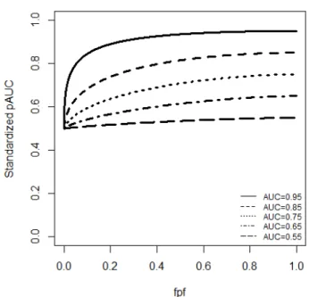
Figure 3.1 Values of the standardized partial AUC for concave binormal ROC curves. ... 28
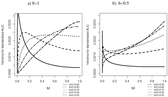
Figure 3.2 Variance of standardized pAUC(0,e) estimates for binormal ROC curves as a function of the size of the range of interest e. ... 31
Figure 3.3 Variance of standardized pAUC estimates for straight-line ROC curves over (0,e) as a function of the size of the range of interest e. ... 31
Figure 3.4 Empirical ROC curves for the two datasets ... 48
Figure 4.1 b=1 and lower AUC=0.8 ... 55
Figure 4.2 Difference in pAUCs for ROC curves of interest (left) vs. Difference in pAUCs for straight-line ROC curves (right) ... 57
Figure 4.3 Bi-gamma ROC curves with AUC=0.8 ... 67
Figure 4.4 Binormal ROC curve (b=1), Bi-gamma ROC curve (κ=1) and a straight-line ROC curve with AUC=0.8 ... 74
Figure 4.5 Empirical estimates of correlated ROC curve from example #1 ... 76
Figure 5.1 Concave binormal ROC curves ... 81
Figure 5.2 Partial concave binormal ROC curves with mass at FPF equal 0.5 ... 82
1.0 INTRODUCTION
1.1 BACKGROUND
A basic problem in evaluation of diagnostic performance involves assessment of the accuracy of a diagnostic test in identifying a patient with a specific, predefined condition (abnormal subject) and a patient without the condition (normal subject). The true status (presence or absence of the abnormality in question) of a subject is assumed to be known for all subjects used for accuracy evaluation. The diagnostic test results can be measured using a binary scale indicating that the subject is assessed as “positive” or “negative”, or an ordinal multi-category (e.g. 7) scale typically with larger values representing higher probability of the abnormality being present, or a continuous scale indicating the likelihood of a pre-specified abnormality being present. For a multi-category diagnostic test, a subject can be classified into a “positive” or “negative” class according to whether the test result is greater than or less than a pre-specified threshold. The Receiver Operating Characteristic (ROC) analysis is the most widely used methodology to investigate this type of research objectives.
ROC analysis originated from signal detection theory (Green and Swets, 1966) (Egan, 1975) and has been well developed over the past 50 years in particular as related to diagnostic imaging and decision making (Metz, 1989) (Hanley, 1989) (McNeil et al., 1975) (Zhou et al., 2002). However, many issues remain and new methods are constantly being developed.
The ROC curve is the plot of sensitivity versus 1-specificity for all possible decision threshold values of c (Figure 1.1). Let X and Y denote the ratings for normal and abnormal subjects respectively. Sensitivity, or true positive fraction (TPF), is the probability of test results being positive for abnormal subjects, and can be defined as follows:
( )
( )
Pr(
)
sensitivity c =TPF c = Y >c
Specificity, or true negative fraction (TNF), is the probability of test results being negative for normal subjects, and can be defined as follows:
( )
( )
Pr(
)
specificity c =TNF c = X ≤c
Figure 1.1 ROC curve
The most commonly used summary index associated with the ROC curve is the area under the ROC curve (AUC). It is defined as
( )
1
0
A=
∫
ROC f dfThe AUC has several interpretations. First, it can be interpreted as the weighted average value of sensitivity of all possible values of specificity (Zhou et al., 2002), or the weighted
also interpreted as the probability that a test result for a randomly selected abnormal patient indicates a greater suspicion of disease than the test result for a randomly selected normal patient (Hanley and McNeil, 1982) (Bamber, 1975). If X and Y are continuous (i.e., no ties in results are possible), then the AUC can be defined as Pr
(
Y >X)
. The value of AUC of 1 indicates a perfect system whereas the non-informative (i.e., guessing) diagnostic system would have AUC of 0.5. An unbiased non-parametric AUC estimate is the area under the empirical ROC curve which is the same as the Mann-Whitney form of the two-sample Wilcoxon rank-sum statistic (Shapiro, 1999). A number of parametric and non-parametric methods based on AUC have been developed to make statistical inferences (Zhou et al., 2002) (Pepe, 2003).AUC offers a single value to indicate the accuracy of diagnostic performance by considering both sensitivity and specificity across all possible threshold values; its major limitation is that it summarizes the entire ROC curve including the region which may not be of interest or practical relevance, for example, the region with very low specificity levels.
To remedy this limitation, partial area under the ROC curve (pAUC) can be used to describe the intrinsic accuracy of diagnostic tests in the range of practical (clinical) interest. The pAUC is frequently defined as
( )
2 1 2 1 , e e e e A =∫
ROC f dfIn practice, a range of
( )
0,e is often used due to the importance of high-specificity range in practice (McClish, 1989) (Jiang et al., 1996). Since the pAUC over an arbitrary interval(
e e1, 2)
is equivalent to the difference in pAUC(0,e2) and pAUC(0,e1) , 0( )
e e
A =
∫
ROC f df will be in focus of my work.A number of statistical methods and inferences based on the pAUC using both parametric and non-parametric approaches have been developed. These include the parametric estimator of the pAUC and its variance using the bi-normal model (McClish, 1989) (Jiang et al., 1996). Wieand et al. (1989) proposed a non-parametric method for estimating pAUC and its variance. Based on Delong’s approach (DeLong et al., 1988), Zhang et al. (2002) proposed a simpler method to compute the variance of pAUC which was subsequently improved by He and Escobar (2008). An alternative nonparametric variance estimator of the pAUC using its expected value was proposed by Liu et al. (2005). Other non-parametric methods have been developed such as empirical likelihood methods, for comparing two pAUCs (Huang et al., 2012) (Qin and Zhou, 2006) (Chen and Wong, 2009), and semi-parametric regression approaches on pAUC by Dodd and Pepe (2003) and Cai and Dodd (2008). However, several conceptual and analytical difficulties prevent pAUC from being widely used.
In general, parametric approaches offer improved efficiency of statistical inferences, but could introduce substantial bias if the needed parametric assumptions are not satisfied. Under the correctly specified model the relative efficiency of nonparametric estimates of partial AUC can be as low as 50% for short ranges of interest (e.g., 0-0.05), but increase beyond 80% efficiency for ranges wider than 0-0.2 (Dodd and Pepe, 2003). For the full AUC, results of parametric and nonparametric inferences are very similar (Hajian-Tilaki et al., 1997) (Hajian-Tilaki and Hanley, 2002). However, it is not always easy to verify appropriateness of the parametric assumptions, and for mis-specified models parametric estimates of pAUC could easily have bias as high as 40% (e.g., Dodd and Pepe, 2003). For this reason it is often recommended to use non-parametric approaches for inferences about partial AUC (Dodd and Pepe, 2003) (Zhang et al., 2002) (He
One of these difficulties is that the scale of values of pAUC increases with increasing range of interest. To partially overcome this limitation, several partial area indices have been proposed (Zhou et al., 2002) (McClish, 1989). A natural transformation of the partial area aimed to “standardize” the range of its values can be written as follows (McClish, 1989):
( )
2 2 0 2 2 2 1 2 1 1 1 2 2 2 2 e e e e ROC f df e A A e e e e − − = + = + − − ∫
(1.1)Here, we term this index as the “standardized partial AUC” (spAUC). For ROC curves describing better-than-chance performance, Ae varies from 0.5 to 1 regardless of e, and for e=1 it reduces to the conventional AUC.
Second, the relevant range should be pre-specified during study design but it is often difficult to determine a priori. In addition, it is often assumed that because of the use of less information, analysis based on the pAUC may result in the loss of statistical precision as compared with statistical inferences based on the full AUC, and thus its use may require larger sample sizes (Zhou et al., 2002) (Obuchowski and McClish, 1997) (Wieand et al., 1989). Conjectures about the relative stability of the spAUC with respect to the range of interest and the decrease in variance with increasing range are intuitively appealing and could affect the way statistical analysis is planned and interpreted. In analyzing experimentally ascertained datasets from observer performance studies we frequently encountered scenarios that contradicted the two conjectures. The work presented here primarily focuses on the investigation of properties of statistical inferences based on the pAUC.
In diagnostic radiology, it is natural to observe multiple subjects having the same diagnostic test results (a tie), in particular at the lowest range, even when the original scale is
continuous or pseudo-continuous (e.g. 0-100 confidence rating scale). A tie at the lower rating could reflect an important characteristic such as the prevalence of the obviously “normal” subjects (e.g., chest images) in a sample, or frequency of the natural absence of a tested substance (Schisterman et al., 2006), or assigning default value to subjects with biomarker levels below a certain limit of concentration and/or a limit of detection (Perkins et al., 2007). When these multiple ties occur at the lowest rating level, the ROC curve includes a straight line segment joining the point corresponding to the lowest threshold and the corner point (1, 1). Since this type of test results has a spike (mass) at the lower threshold, for brevity we term such a curve as an “ROC curve with mass”. For the ROC curve with mass, a parametric mixed model combined with Box-Cox transformation and a non-parametric approach based on the Mann-Whitney statistic for the estimation of AUC has been proposed and discussed (Schisterman et al., 2006). The parametric mixed model approach can be further used to estimate Youden’s Index and determine the optimal threshold for test results with mass (Schisterman et al., 2008). However, issues related to the evaluation of a single pAUC and the comparisons of two correlated pAUCs associated with ROC curves with mass remain unsolved to date.
1.2 OBJECTIVES
The emphasis of this dissertation will be on investigations of statistical properties when evaluating diagnostic performance using pAUC. We believe that in many practical scenarios inferences based on pAUC could be no less statistically advantageous than inferences based on the full AUC. Thus the use of pAUC may actually lead to not only more relevant but also more
studies. This should encourage researchers and practitioners to more frequently apply this highly relevant, but currently underused summary index. The results of our investigation could also provide foundation for decisions about optimal thresholds to achieve greatest statistical power and therefore smaller sample sizes when using pAUC.
This dissertation includes the following three objectives.
Objective 1:
As related to evaluation of a single diagnostic system, we investigate the effect, if any, of the range of interest
( )
0,e on statistical inferences when the pAUC(0,e) is used as a summary measure of performance. We analyze the properties of nonparametric and parametric estimates of standardized pAUCs and their variances. Using extensive simulation studies, we investigate the statistical power for different families of ROC curves such as binormal ROC curves, bi-gamma ROC curves and straight-line ROC curves. Based on the results of this research, we develop a program for estimating sample size in the evaluation of a single pAUC in a range of practically relevant scenarios.Objective 2:
We extend the developments from objective 1 for the task of comparison of accuracy levels of two diagnostic systems on the basis of pAUC computed from the paired data collected with each case rated under every modality. First, we analytically investigate conditions for the increasing difference in the standardized pAUC with increasing size of the range of interest. Based on extensive simulation studies, we investigate the statistical power for comparisons of pAUCs over different ranges of interest under the ROC scenarios (such as binormal ROC curves, bi-gamma ROC curves and straight-line ROC curves) which lead to different patterns of changes in pAUC with increasing range. Based on the result of this research, we develop a program for
estimating sample size for comparison of two correlated pAUCs for a variety of practical scenarios.
Objective 3:
The task of evaluation of diagnostic modalities is often complicated by presence of substantial ties in the data. Using mathematical considerations and extensive simulations, we investigate the properties of the differences in the pAUCs and statistical power over different ranges of interest. The expectation is that the trends of increasing/decreasing variance with increasing range of interest would become less pronounced for data with ties at the lowest rating value (corresponding to the ROC curve with mass) as compared with data without ties. This could affect the expected patterns in statistical power. The results of this investigation will help plan the analyses of diagnostic accuracy using data with ties at the lowest rating levels and make more informative decisions about the data collection protocols.
2.0 FACTS RELATED TO THE PRESEARCH
2.1 FAMILIES OF ROC CURVE, THEIR AUCS AND PAUCS
2.1.1 BINORMAL ROC CURVES
Bi-normal ROC curve is the most widely used model in ROC analysis (Zhou et al., 2002). The name “binormal” reflects the shape of ROC curves and stems from the fact that “binormal” ROC curve can result from the two (independent) normally distributed random variables. However, the use of the binormal ROC curve does not necessarily imply that the test results are assumed to follow normal distributions in the subpopulation of normal and abnormal patients. Rather, the use of a binormal ROC curve implies that the observed diagnostic result is related (according to a certain monotonically increasing transformation, with possible grouping for discrete case) to normally distributed latent scores.
For a pair of latent scores for normal and abnormal patients which follow two normal distributions, i.e.
(
2)
~ x, x
X N µ σ and
(
2)
~ y, y
Y N µ σ respectively, the ROC curve can be expressed as:
( )
(
1( )
)
where
(
y x)
y a µ µ σ − = x y b σ σ= and Φ is the cumulative normal distribution function. This
relationship between
( )
a b, and the parameters of the distribution of the latent scores is rarely used in practice. One of the exceptions is to fit the ROC curve for continuous data using Box-Cox transformation (Zou and Hall, 2000); however, this relationship is very useful in simulation studies.The AUC for the binormal ROC can be expressed as:
( )
(
)
1 1 2 0 1 a A a b x dx b − = Φ + Φ = Φ + ∫
and the pAUC as:( )
(
1)
0 e e A = Φ + Φ∫
a b − x dxHillis and Metz provided an analytic expression for pAUC in the case of binormal ROC curves (Hillis and Metz, 2012),
( )
1 2 , ; 2 1 1 e BVN a b A F e b b − = Φ − + + where FBVN
(
z x, ;ρ)
is the standardized bivariate normal distribution function with correlationρ.2.1.2 POWER-LAW ROC CURVES
Another well-known, but simpler and less flexible (due to a single-parameter type) family of ROC curves is described by the “power-law” curves (Egan, 1975) (Hanley, 1988), or Lehman family of the ROC curves (Gonen and Glenn, 2010). One of the reasons to consider this model
1988) and enabling simple inferences using built-in software (Gonen and Heller, 2010). Power-law ROC curve can result from two exponentially distributed variables. However, the use of the power-law ROC curve does not necessarily imply that the test results are assumed to follow exponential distributions in the subpopulation of normal and abnormal patients. Rather, similar to other parametric ROC curves, the use of a power-low ROC curve implies that the observed diagnostic result is related (according to a certain monotonically increasing transformation, with possible grouping for discrete case) to exponentially distributed latent scores.
For a pair of latent scores for normal and abnormal patients which follow two exponential distributions, i.e. X ~Exp
( )
θx and Y ~Exp( )
θy respectively, the ROC curve (power-law) can be expressed as:( )
exp x y ROC e θ e θ = . with the AUC of:1 0exp exp 1 y x x y x y A θ f df θ θ θ θ θ = = −
∫
,and the pAUC of:
1 0exp exp 1 y x x e y x y A θ x dx θ θ e θ θ θ = = −
∫
.2.1.3 BI-GAMMA ROC CURVES
Bi-gamma family is another of the well-known families of the ROC curves (Egan, 1975) (Dorfman et al., 1996) (Faraggi et al., 2003) (Huang and Pepe, 2009). In general bi-gamma ROC
curves constitute a three-parameter family, however, in practice a subfamily of concave curves represented by “constant-shape bi-gamma ROC curves” is used (Dorfman et al., 1996). Similar to the binormal ROC curves, the constant shape bi-gamma ROC curves constitute a two-parameter family, however, it offers more flexible shapes of the practically reasonable concave ROC curves (a subfamily of concave binormal ROC curve is a one-parameter family).
The primary disadvantage of bi-gamma ROC curve lies in the relative complexity of computations. However, the computational complexity is alleviated with the development of software packages and theoretical investigations of the properties of bi-gamma ROC curves (Constantine et al., 1986). A bi-gamma ROC curve can be parameterized with parameters of the gamma distribution of the latent (as opposed to actual) ratings for normal and abnormal subjects. We note that similar to other ROC models, the underlying assumption of a bi-gamma-type shape of the ROC curve does not imply an assumption of a bi-gamma distribution of the actual ratings (due to the invariance of the ROC curve with respect to monotonically increasing transformation of the ratings). In other words, the distributions of latent ratings are simply intermediate steps for parameterization of the ROC curve. The probability density function of the underlying rating model of the bi-gamma ROC curve has the following form:
( )
1 1 1 ( ; , ) x k k f x k x e k θ θ θ τ − − = ,In general parameters θ and κ could be different for the latent normal and abnormal ratings. The constant-shape bi-gamma ROC curves are obtained by constraining the shape parameter κ to be the same for two distributions. When κ approaches 0, the bi-gamma ROC curve approaches the shape of a straight-line and when κ>1 the shape of the bi-gamma ROC
normal distribution when shape parameter κ is large (We note however, that this does not guarantee convergence of the ROC curves). When κ=1 the bi-gamma ROC curve is equivalent to the power-law ROC curve (Egan, 1975) (Hanley, 1989).
For a pair of latent scores for normal and abnormal patients which follow two gamma distributions, i.e.X ~Gamma
(
θ κx, x)
and Y ~Gamma(
θ κy, y)
respectively, the ROC curve can be expressed as:( )
(
1( )
)
y x
ROC e =S S− e .
The density of the Gamma distribution is given by
( )
1 1 1 ( ; , ) x k k f x k x e k θ θ θ τ − − = and S denotesthe survival function of Gamma distribution.
Due to the relationship between Gamma and Beta distribution the AUC of the bi-gamma ROC curve can then be expressed (Constantine et al., 1986) (Hussain, 2012) as:
(
)
0 1(
)
1 F(
(
)(
)
)
1 1 1 ; 2 , 2 ; , , y y x x y y y x x y y x beta x y x y y x A x x dx F F B θ κ κ θ θ κ κ θ θ κ κ θ κ κ θ θ κ κ − − + = − = − = + ∫
where FF
(
*; 2κy, 2κx)
is the cumulative distribution function (CDF) of an F random variable with parameters2κyand 2κx, and Fbeta(
*;κ κx, y)
is the CDF of a beta random variable with parameters κx and κy.As of now there are no simplified expressions for the pAUC, and it is usually computed using numerical integration according to the original definition:
( )
(
1)
0 e e y x A =∫
S S− e dx.2.1.4 STRAIGHT-LINE ROC CURVES
We define a “straight-line” ROC curve as the curve consisting of two line segments the vertical segment connecting the point (0, 0) and the point (0, 1/a), where a>1, and a line segment connecting the point (0, 1/a) and the point (1, 1). Namely:
ROC e
( )
1e 1 1a a
= + − (2.1) Such a curve describes a theoretically important scenario where diagnostic result perfectly separates the most obvious “abnormal” patients, while being non-informative for discriminating between normal and abnormal patients in the remaining population. Indeed, using a flip of a coin it is possible to create a diagnostic test with operating characteristics anywhere on the straight line extending to (1, 1) (Wagner et al., 2010) (Bandos et al., 2010). Theoretical importance of this type of a ROC curve for the current work stems from the ancillary nature of the operating points with non-zero FPF. In practice the pure straight-line ROC curves (i.e., with empirical points aligned around the straight line) could occur when a diagnostic system is forced to produce continuous (untied) results in situations when there is little or no information for distinguishing between subjects (Gur et al., 2006).
Straight-line ROC curve has a constant value of standardized partial AUC regardless of the range of interest (Ma et al., 2013); this offers an important scenario for investigating pAUC-based inferences.
The name “straight-line” simply reflects the shape of the curve. The ROC curve with a straight-line shape would result from the two (independent) random variables with uniform distributions. However, due to the ROC invariance property the use of the straight-line ROC
in the subpopulation of normal and abnormal patients. In general it can be viewed as a curve corresponding to a diagnostic result that perfectly separates the most obvious “abnormal” patients, while is non-informative for discriminating between normal and abnormal patients in the remaining population.
For a pair of latent scores for normal and abnormal patients which follow two uniform distributions, i.e.X ~U
( )
0,1 and Y ~U( )
0,a respectively, the ROC curve can be expressed as:( )
1 11
ROC e e
a a
= + − .
and the AUC can be expressed as
1 0 1 1 1 1 1 2 A e dx a a a = + − = −
∫
,while the pAUC can be expressed as:
2 0 1 1 1 1 1 1 2 e e A e dx e e a a a a = + − = − +
∫
.2.2 ESTIMATION OF ROC CURVES
2.2.1 PARAMETRIC ESTIMATES OF ROC CURVES
A number of approaches exist for parametric estimation of the ROC curve. The two general classes of parametric estimation methods are “distribution-free” and “distribution-based” approaches.
Distribution-free approaches may place parametric assumption on the shape of the ROC curve, e.g., binormal ROC curve,ROC e
( )
= Φ(
a b+ Φ−1( )
e)
, but not on the distributions of scores for diseased and non-diseased subjects. For continuous test results, Pepe (2003) proposed an estimation method involving the methods of generalized estimating equations and generalized linear models which can incorporate covariate information. Zou and Hall (2000) performed MLE rank-based estimation of binormal ROC curves. For discrete test results, a maximum likelihood approach was introduced by Dorman and Alf (1969).Distribution-based approaches, on the other hand, estimate conditional distribution of the test results (given subjects’ true status); the ROC curve is then estimated indirectly as the composition quantile and distribution function. For example, a naïve distribution-based approach for estimating the binormal ROC curve (which is rarely used in practice), assumes a normal distribution of the test results. If X and Y are the test results for the random samples of m normal and n abnormal subjects, based on the invariance principle, the maximum likelihood estimate (MLE) of the binormal ROC curve can be expressed as follows (Zhou et al., 2002):
( )
(
ˆ 1( )
)
ˆ ˆ ROC e = Φ a b+ Φ− x where ˆ(
ˆ ˆ)
ˆ y x y a µ µ σ − = , ˆ ˆ ˆ x y b σ σ= , ˆµx, µˆy, ˆσx and σˆy are the ML estimates of the means and
standard deviations, and Φ is the cumulative normal distribution function. Given that the binormal distribution assumption is restrictive and based on the invariance property of monotonic transformation of ROC curves, Faraggi et al. (2003) applied a Box-Cox type power transformation to the data, and after obtaining the appropriate transformation used binormal model.
2.2.2 EMPIRICAL ROC CURVE
The empirical ROC curve is a collection of the empirical operating points (FPFˆ and TPFˆ ) where The empirical true and false positive fractions are computed as follows:
( )
1 ˆ n j j I Y c TPF c n = > =∑
,( )
1[
]
ˆ m i i I X c FPF c m = > =∑
.where I x
( )
=1 if x is true and 0 otherwise. However, frequently the empirical ROC curve is plotted by connecting the empirical points with straight line segments. Some analytical methods however, do not use the points on the straight-lines (Greenhouse and Mantel, 1950) (Wieand et al., 1989) (Zhang et al., 2002) (He and Escobar, 2008). The points on the straight-line segments between the empirical points describe operating characteristics which might not be attainable by applying specific thresholds to the observable test results. However, these could be attained by random guessing between the decisions at the adjacent operating points (Fawcett, 2006) (Wagner et al., 2010) (Bandos et al., 2010).We will use the term “linearly-interpolated” empirical ROC curve to distinguish it from the set of discrete
(
fpf tpf,)
points.2.3 ESTIMATION OF AUC AND PAUC
2.3.1 PARAMETRIC ESTIMATES OF AUC AND PAUC
Parametric analyses based on AUC and partial AUC are reasonably straightforward. The previously mentioned methods can be used to estimate smooth ROC curves. Once a smooth curve is fitted, the partial area can be estimated for any specified range of interest; its variance can be evaluated using the “delta” method based on the variance of the model parameters (Zhou et al., 2003). For naïve binormal model, the estimated AUC or partial AUC can be computed as follows:
( )
(
)
1 1 0 2 ˆ ˆ ˆ ˆ ˆ 1 a A a b x dx b − = Φ + Φ = Φ + ∫
( )
(
1)
0 ˆ ˆ e ˆ e A = Φ + Φ∫
a b − x dx where ˆ(
ˆ ˆ)
ˆ y x y a µ µ σ − = , ˆ ˆ ˆ x y b σ σ= , ˆµx, ˆµy, ˆσx and ˆσyare the MLE of the mean and standard
deviations of the latent scores (e.g., MLE estimates for a and b can be obtained from the probit regression model of the discrete test results), and Φ is the cumulative normal distribution function. Or by using analytic expression for pAUC in the case of binormal ROC curves (Hillis and Metz, 2012),
( )
1 2 2 ˆ ˆ ˆ , ; ˆ ˆ 1 1 e BVN a b A F e b b − = Φ − + + 2.3.2 EMPIRICAL ESTIMATES OF AUC AND PAUC
If
{ }
Xi im=1 and{ }
1 n j j Y= are the test results for random samples of m normal and n abnormal
subjects then the estimate of the AUC can be expressed as follows:
1 1 ( , ) ˆ m n i j i j X Y A nm ψ = = =
∑∑
where(
)
1 2 1 , 0 X Y X Y X Y X Y ψ < = = > This non-parametric AUC estimator is equal to the area under the empirical ROC curve where the points on the plot are connected by straight lines.
The partial area can be estimated by (He and Escobar, 2008):
(
)
1 1 1 ˆ m n , e i j i j A X Y mn = = φ =∑∑
where(
)
0 0 0 1, [ , ) 1 , , [ , ) 2 0, [ , ) j i i i j j i i j i i Y X and X r X Y Y X and X r Y X and X r φ > ∈ ∞ = = ∈ ∞ < ∈ ∞ (
)
1 0 x 1 r =F− −eand Fx is the empirical distribution of Xi.
For any consecutive ratings r1andr2 where r2 <r1, e1=FPF r
( )
1 and e2 =FPF r( )
2 , if(
1, 2)
e∈ e e , one can a use linear interpolation to compute the pAUC which can be expressed as follows:
( ) (
)
(
(
( )
)
( )
)
(
)
1 1 2 1 1 1 2 1 ˆ ˆ 2 e e e e TPF r TPF r A A TPF r e e e e − − = + + − − .2.4 ESTIMATION OF VARIANCE OF AUC AND PAUC
In general variance of the parametric AUC and pAUC estimators can be obtained from a variance matrix of the estimated parameters (corresponding to the ROC fitting approach) using delta method (Zhou et al., 2002). For the naïve fitting of the binormal ROC curve (assuming normally distributed test result) the variance estimator attains the following closed-form expression in terms of a and b parameters of the binormal model (Obuchowski and McClish, 1997): V Aˆ
( )
ˆe = f V a2( )
ˆ +g V b2( )
ˆ +2fgC a b( )
ˆ, ˆ (2.1) where:( )
(
2 2)
2 2 ˆ ˆ 2 m a nb V a mn + + =( )
(
)
2 ˆ ˆ 2 n m b V b mn + =(
)
(
)
{
( )
}
2 2 2 exp 2 1 2 1 a b f h b π − + = Φ +( )
ˆ ˆ ˆ, 2 ab C a b n = and( )
1 2 2 1 1 ab h e b b − = Φ + + + Due to the close relationship to the Mann-Whitney test statistics (Bamber, 1975), variance of the AUC estimator for an empirical ROC curve can be derived from the formula for the Wilcoxon statistics proposed by Noether (1967):
10 01 11 1 1 1 ˆ ( ) m n Var A mn ξ mn ξ mnξ − − = + + ∀i k, =1,...,m j l, =1,...,n where
{
(X ,Y ), (X ,Y )} {
E (X ,Y ) (X ,Y )}
A , j l Cov i j i l i j i l 2 10 = ψ ψ = ψ ψ − ≠ ξ{
} {
}
2 01 Cov (X Yi, j), (X Yk, j) E (X Yi, j), (X Yk, j) A , i k ξ = ψ ψ = ψ ψ − ≠{
}
{
2}
2 j i j i 11 =Varψ(X ,Y )= Eψ(X ,Y ) −A ξ{
( , )}
{ }
ˆ i j A=E ψ X Y =E AFor continuous test results which are often encountered in many scenarios such as genetic research, He and Escobar (2008) proposed a non-parametric variance estimator for the partial area. Alternatively, the variance of empirical estimators of AUC and pAUC can also be estimated using a nonparametric bootstrap approaches (Efron and Tibshirani, 1993). The variance can be estimated by resampling the normal and abnormal subjects and linearly interpolating the empirical ROC curves. Another variance estimator of the pAUC using a non-parametric approach was proposed by Liu et al. (2005). If
{ }
Xi im=1 and{ }
1
n j j Y
= are the test results
for random samples of m normal and n abnormal subjects with distribution functions Fxand Fy, and empirical distribution functions Fxand Fyrespectively, then the asymptotically unbiased estimator ˆAeof pAUC can be expressed as:
(
)
( )
1 1 1 ˆ n e j i y i j i i A I Y X S X mn = ∈Ρ m ∈Ρ =∑∑
> =∑
where Sy
( )
z = −1 Fy( )
z , Ri is the rank of Xi among the X’s, that is,(
)
1 m i k i k R I X X = =∑
≤ , and{
i m: (1 e) Ri m}
Ρ = − ≤ ≤ . They also showed that:
2 ˆ d , e e e A N A m n σ → + Where: 2 2 2 / / e H W σ =σ λ σ′+ λ
(
)
(
)
1 1 2 1 2 1 1 W e eSy Fx s t dsdt Ae σ − − − =∫ ∫
∨ − ,( )
max , s∨ =t s t ,( )
(
)
1 2 2 1 2 1 H eSy Fx p dp Ae σ − − =∫
− ,(
)
1 m m n λ′ = − =λ + ,( )
1( )
x x S z = −F z andSy( )
z = −1 Fy( )
z .Moreover, the consistent estimators of σH2 and σW2 , respectively can be obtained:
( )
{
}
2 2 1 ˆ2 ˆH y i e i S X A m σ ∈Ρ =∑
− ,(
)
(
)
2 1 ˆ2 ˆ 1 W y i k e i k S X X A m m σ ≠ ∈Ρ = ∨ − −∑
.3.0 EVALUATION OF A SINGLE PAUC
The statistical inference regarding diagnostic accuracy of a single modality (diagnostic system, classification tool, etc.) is often made on the basis of summary indices such as pAUC and AUC. For example, diagnostic accuracy for classifying images as depicting or not-depicting lung nodules can be assessed using both point estimation and interval estimation of pAUC and AUC. In the evaluation of a single pAUC, we investigated the effect of the size of the range of interest (0, e) on statistical inferences regarding the pAUC. We analyzed the properties of the nonparametric and parametric estimates of spAUCs and their variances. We derived two important properties of the relationship between the spAUC and a defined range of interest, which could facilitate a wider and more appropriate use of this important summary index. First, we mathematically proved that the spAUC increases with increasing range of interest for common ROC curves. Second, using a comprehensive numerical investigation we demonstrated that, contrary to common belief, the uncertainty about the estimated spAUC can either decrease or increase with an increasing range of interest.
Our results indicated that the pAUC could offer advantages in some scenarios in terms of statistical uncertainty of the estimation. In addition, selection of a wider range would likely lead to an increased estimate even in the case of spAUC. We demonstrated that the bi-gamma family of the concave ROC curves adequately describes a wide range of scenarios including cases where pAUC is statistically advantageous. This family was used to develop sample size
estimation software offering a better insight in relative merits of analyzing part of the curve. This portion of the research is published in Statistics in Medicine (Appendix A).
3.1 METHOD
3.1.1 STANDARDIZED PARTIAL AUC AND ITS PROPERTIES
Based on the definition of standardized pAUC (1.1), it can be shown that the standardized pAUC and the variance of its estimate are always larger than conventional pAUC and the variance of its estimate. Indeed since 1/e/(2e-1), is less than 1 for all e≤1:
2 2 1 1 1 2 2 2 2 2 e e e e e e A ≥ + A − = A + − ≥A and
( )
( )
2 2( )
ˆ ˆ ˆ 4 2 e e e e V A =V A e− ≥V A .Unfortunately, “standardization” of the partial area in (1.1) is not ideal. Indeed, although the range of Ae is independent of e, the actual value of Ae for a given ROC curve could depend on e. Moreover, as we demonstrate in Proposition 3.1 below, theoretically it can either increase or decrease with increasing range while remaining constant only in the case of a “straight-line ROC curve” (Chapter 2.1.4) composed of two straight-line segments – one vertical and the other passing through the point (1,1). Using equation (2.1) it is easy to see that partial AUC for the straight-line ROC curve passing through the point
( )
f t, is:( ) 2
(
) (
)
{
(
) (
)
}
, , , 1 2 1 1 1 1
e straight f t
A =e −t − f +e − −t − f
and the standardized partial AUC does not depend on the range of interest (independent of e):
( )
(
) (
)
, , 1 1 2 1 straight f t A = − −t − f (3.1) Proposition 3.1 For any e∈( )
0,1 , i. Ae e ∂ ∂ 0 > ⇔ ROC e( )
>2 1(
−A ee) (
+ 2Ae−1)
ii. Ae e ∂ ∂ 0 = ⇔ ROC e( )
=2 1(
−A ee) (
+ 2Ae−1)
iii. Ae e ∂ ∂ 0 < ⇔ ROC e( )
<2 1(
−A ee) (
+ 2Ae−1)
Proof:By straightforward differentiation of (1.1) we obtain:
( )
(
)
(
)
2 2 2 2 1 1 2 2 2 2 e e A e e e e ROC e e e A e e − ∂ = − − − − − − ∂ Since(
)
2 2 2 1 2 2 e e e e A − = A − e− , the derivative of standardized partial AUC can be
written as follows:
( )
(
)
(
)
(
)
{
}
1 2 1 2 1 1 2 2 e e A e e ROC e e A e e − ∂ = − − − − − ∂ The three claims of this proposition immediately follow.
Proposition 3.1 implies that given the area over the range (0,e), we can determine whether a small increase in the range would lead to an increase in the standardized pAUC by comparing whether the point on the ROC curve ROC(e) is actually above or below the fixed
straight line, that passes through the point (1,1) and has a slope of 2 1
(
−Ae)
. Alternatively, this comparison can be conducted by comparing the negative diagnostic likelihood ratio (1-ROC(e))/(1-e) with 2 1(
−Ae)
.The negative diagnostic likelihood ratio, DLR-(e), is an important characteristic of binary diagnostic test (Zhou et al., 2002) (Norman, 1964) (Biggerstaff, 2000) (Bandos et al., 2010). For a point on the ROC curve (e,ROC(e)) it is defined as (1-ROC(e))/(1-e). The ROC curve with a decreasing negative diagnostic likelihood ratio is practically important. Such an ROC curve ensures that starting at any given operating point, a threshold-driven improvement in sensitivity will be better than an improvement achieved by randomly selected subjects that were tested “negative” at the given operating point (Norman, 1964) (Bandos et al., 2010). Thus, a decreasing negative diagnostic likelihood ratio in the region where experimental operating points are observed is a natural property for many practical diagnostic tests.
While results of proposition 3.1 are important for judging the dependence of spAUC on small changes in the range of interest, they provide little insight into the more global behavior of the spAUC, or the general form of curves with always increasing/decreasing Ae. These questions are addressed by the following proposition and its corollaries.
Proposition 3.2
If the ROC curve has a decreasing negative diagnostic likelihood ratio in (0, e0), namely,
( )
1 0 1 ROC e e e − ∂ < ∂ − , then 0 e A e ∂ > ∂ in the same range. Proof:
Let us consider e from
(
0,e0)
. Since for any e`∈(0,e) 1( )
` 0 1 f e ROC f f f = − ∂ < ∂ − , wecan obtain the following inequality :
( )
( )
( )
(
)
( )
1 1 ` 1
` 1 1 `
1 1 ` 1
ROC e ROC e ROC e
or ROC e e
e e e
− − −
< < − − ×
− − −
Hence over the range (0, e], the partial area (Ae) and the standardized partial area under the ROC curve
( )
Ae are smaller than the corresponding areas under the straight line ROC curve passing though (e, ROC (e)). Indeed:( )
(
)
( )
, ,( , ( )) ,( , ( )) 0 0 1 1 1 . 1 e ee e straight e ROC e e straight e ROC e ROC e A ROC f df f df A A A e − = < + − × = ⇒ < −
∫
∫
On the other hand, from (2) we have:
( )
2 1(
straight e ROC e,( , ( )))
(
2 straight e ROC e,( , ( )) 1)
2 1(
)
straight e ROC e,( , ( )) 1.ROC e = −A e+ A − = −e A +
Also, since Ae <Astraight e ROC e,( , ( )), from above we obtain:
( )
2 1(
)
e 1 2 1(
e) (
2 e 1)
ROC e > −e A + = −A e + A −
Finally, applying the result (i) of proposition 3.1 we obtain Ae 0
e ∂ > ∂ .
As we discussed previously in this section, a decreasing negative diagnostic likelihood ratio is a natural property for many practical diagnostic tests. We also note that the result of proposition 3.2 is directly applicable to concave ROC curves, as it can be demonstrated that concavity immediately implies a decreasing diagnostic likelihood ratios. Figure 3.1 illustrates the increase of the standardized partial AUC with increasing range for five concave binormal ROC curves.
Figure 3.1 Values of the standardized partial AUC for concave binormal ROC curves.
We note that proposition 3.2 is directly extendable to the partial area index (McClish, 1989) (Jiang et al., 1996) as well as to the “non-standardized” partial area. Results summarized in this section indicate that in practical scenarios, current approaches to standardization of the partial AUC do not necessarily eliminate the effect of the range of interest on values of the standardized pAUC. Moreover, increasing range of can frequently increase the apparent level of diagnostic performance. In the next two sections we examine the statistical uncertainty in the estimated standardized partial AUC.
3.1.2 VARIANCE OF THE PARAMETRIC ESTIMATE OF SPAUC
correspondingly. We focus here on the relationship between the variance of the spAUC and the size of the range of interest. In particular, we examine the common conjecture that variance would decrease with increasing range, since a larger range incorporates more available information in regards to the operating characteristics.
We begin by considering a simple variance estimate for the partial area under the binormal ROC curve (McClish, 1989). Then, in section 5 we present simulation results that demonstrate the generality of the derived conclusions.
We can compute the variance of the estimated standardized partial AUC as:
( )
( )
2 2 ˆ ˆ 4 2 e e V A V A e e = − , where( )
ˆ e V A is computed according to (2.1).Figure 3.2 demonstrates the variance of the estimated standardized pAUC as a function of the length of the range e, for two different binormal as well as straight-line ROC scenarios. These scenarios are based on a sample size of 100, (m=n=50) and describe different shapes of ROC curves, including concave curves (b=1) and typical improper curves (b=0.5) (Obuchowski and McClish, 1997). Each figure shows variance functions for five ROC curves with AUCs of 0.55, 0.65, 0.75, 0.85, and 0.95.We note that here, as well as in the investigations that follow, we consider binormal ROC curves with b≤1 since the corresponding shapes of these ROC curves are more common in practical applications including, but not limited to, medical imaging. Indeed, a binormal ROC curve with b>1 implies a worse-than-chance performance in evaluations of highly suspicious subjects (i.e., in the range of high specificity) – which rarely happens in practice.
For concave ROC curves (Figure 3.2a) the variance of the full AUC can exhibit both patterns, namely, it can be either smaller or larger than variance of the standardized partial AUCs on (0, e). The decrease in variance with increasing range is observed only for ROC curves with
AUC values greater than 0.75. In the straight-line ROC scenarios for which all standardized partial AUCs are exactly the same as the full AUC, the variance of the standardized partial AUC increases. As shown in Figure 3.2b, for an improper binormal ROC curve, the variance frequently increases with increasing range, in particular the variance of the full AUC (e=1) tends to be larger than the variances for standardized partial AUCs over most ranges considered. The anticipated decrease in the variance when switching to full AUC is evident only for the ROC curve with the largest AUC (0.95) considered herein.
a) b=1 b) b=0.5
Figure 3.2 Variance of standardized pAUC(0,e) estimates for binormal ROC curves as a function of the size of the range of interest e.
Figure 3.3 Variance of standardized pAUC estimates for straight-line ROC curves over (0,e) as a function of the size of the range of interest e.
These results provide an important indication that there are a number of practical scenarios in which the estimated partial AUC may be no less precise than the estimated variance for the full AUC. Variance is an important characteristic of the statistical uncertainty, however, its usefulness for non-symmetric distributions is limited (e.g., sampling distribution of estimates of high pAUC). Furthermore, the trends shown in Figure 3.2 are based on the assumption of normality of the test result, and hence might not be generalizable. In order to verify these trends we conducted a simulation study as described in the following section.
3.2 NUMERICAL STUDY
In this section we considered several families of ROC curves including binormal, bi-gamma and straight-line ROC curves. For each scenario, we computed the standardized pAUC by numerical integration. We conducted a simulation study to assess the length of the equal-tail 95% range (97.5th -2.5th percentile) and variance of the sampling distribution of the standardized pAUC. The statistical power was estimated from 1000 results of the bootstrap tests and the sample size was computed by established results for Wald-type tests (Flahault, 2005). In the simulation study the test results for normal and abnormal subjects were generated from normal distributions with parameters selected to generate binormal ROC curves with specific values of AUC (ranging from 0.55 to 0.95) and for three values for the shape parameter b (1, 0.5 and 0.33). Values for the parameters of binormal ROC curves were selected to reflect shapes typically encountered in experimental performance assessment studies in diagnostic medicine. For the bi-gamma ROC curves the test results were generated from gamma distributions with the same shape parameter
uniform distributions of different width. For each scenario we generated 10,000 datasets of with m=50 and n=50 subjects.
For each generated dataset we estimated the empirical ROC curve and, using numerical integration, computed the standardized partial AUC over different ranges starting from 0 and ending at 0.2, 0.4, 0.6, 0.8, and 1. The difference between the 9750th (largest) and 250th (smallest) estimate of the AUC for a given scenario was used to estimate the length of the equal-tail 95% range of the sampling distribution. We note that transformations (e.g., logit) are often used to improve on Wald-type confidence intervals. In the simulation study, however, we have the ability to assess the width of distribution more precisely by using percentiles of the simulated distribution.
Scenario 1:
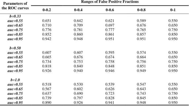
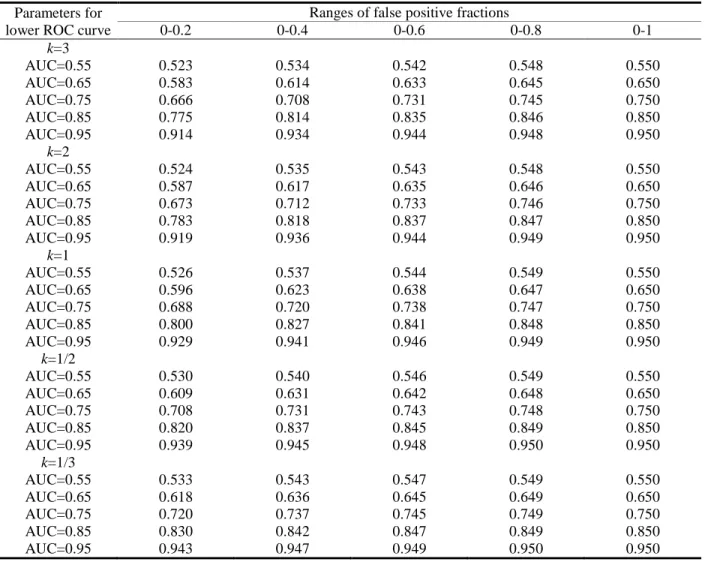
We first investigated the properties of standardized pAUC for binormal ROC curves. Table 3.1 showed that the standardized pAUC increased with increasing range for concave binormal ROC curves and improper ROC curves with high AUC, i.e. b=0.5 AUC≥0.85, and for b=0.33, AUC=0.95.
Table 3.1 Theoretical spAUC for binormal ROC curves with different b’s and full AUCs
Parameters of the ROC curves
Ranges of False Positive Fractions
0-0.2 0-0.4 0-0.6 0-0.8 0-1 b=0.33 auc=0.55 0.651 0.642 0.621 0.589 0.550 auc=0.65 0.710 0.709 0.697 0.676 0.650 auc=0.75 0.776 0.781 0.777 0.765 0.750 auc=0.85 0.852 0.860 0.861 0.857 0.850 auc=0.95 0.942 0.948 0.951 0.951 0.950 b=0.50 auc=0.55 0.607 0.607 0.595 0.574 0.550 auc=0.65 0.665 0.676 0.674 0.664 0.650 auc=0.75 0.734 0.753 0.758 0.756 0.750 auc=0.85 0.818 0.840 0.848 0.851 0.850 auc=0.95 0.926 0.940 0.946 0.949 0.950 b=1.0 auc=0.55 0.518 0.530 0.539 0.547 0.550 auc=0.65 0.567 0.602 0.626 0.643 0.650 auc=0.75 0.637 0.690 0.723 0.743 0.750 auc=0.85 0.739 0.797 0.828 0.845 0.850 auc=0.95 0.890 0.926 0.941 0.948 0.950
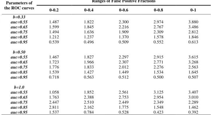
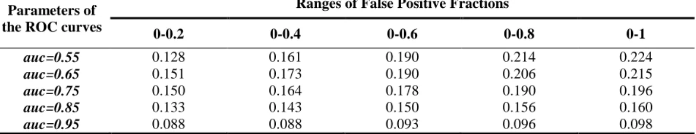
The results for the empirical estimator of the standardized pAUC are summarized in Tables 3.2 and 3.3. These results closely agree with results from the previous section (Figure 4.1). In particular, the variances and lengths of the equal-tail 95% ranges of the sampling distributions of the estimated standardized pAUCs increase with increasing ranges for the ROC curves with lower AUCs (e.g., AUC for concave ROC curves is less than 0.75). With increasing “improperness” of the ROC curves (i.e., decreasing b) decreasing trends, even for ROC curve with large AUCs, are gradually diminishing. For example, for a binormal ROC curve with b=0.33, the variance and length of the equal-tail 95% interval of sampling distribution of standardized pAUC increases with increasing range of interest for all considered ROC curves.
Table 3.2 Variance of sampling distributions of standardized pAUC for binormal ROC curves (×10-3)
Parameters of the ROC curves
Ranges of False Positive Fractions
0-0.2 0-0.4 0-0.6 0-0.8 0-1 b=0.33 auc=0.55 1.487 1.822 2.300 2.974 3.880 auc=0.65 1.599 1.845 2.216 2.767 3.486 auc=0.75 1.494 1.636 1.909 2.309 2.812 auc=0.85 1.212 1.237 1.370 1.578 1.846 auc=0.95 0.539 0.496 0.509 0.552 0.613 b=0.50 auc=0.55 1.467 1.827 2.297 2.915 3.615 auc=0.65 1.723 1.966 2.307 2.771 3.268 auc=0.75 1.776 1.833 2.012 2.276 2.563 auc=0.85 1.539 1.427 1.449 1.534 1.645 auc=0.95 0.718 0.563 0.512 0.500 0.507 b=1.0 auc=0.55 1.058 1.852 2.561 3.125 3.407 auc=0.65 1.763 2.388 2.753 2.954 3.010 auc=0.75 2.447 2.510 2.449 2.349 2.289 auc=0.85 2.811 2.162 1.775 1.548 1.462 auc=0.95 1.537 0.784 0.528 0.423 0.392