Multi-Label Classification Based on
the Improved Probabilistic Neural
Network
Huilong Fan(1), Yongbin Qin(2)
(1) Guizhou Key Laboratory of Public Big Data, Guizhou University, Guiyang, CHINA (2) College of Computer Science and Technology, Guizhou University, Guiyang, CHINA
SUMMARY
This paper aims to overcome the defects of the existing multi-label classification methods, such as the insufficient use of label correlation and class information. For this purpose, an improved probabilistic neural network for multi-label classification (ML-IPNN) was developed through the following steps. Firstly, the traditional PNN was structurally improved to fit in with multi-label data. Then secondly, a weight matrix was introduced to represent the label correlation and synthetize the information between classes, and the ML-IPNN was trained with the backpropagation mechanism. Finally, the classification results of the ML-IPNN on three common datasets were compared with those of the seven most popular multi-label classification algorithms. The results show that the ML-IPNN outperformed all contrastive algorithms. The research findings brought new light on multi-label classification and the application of artificial neural networks (ANNs).
KEY WORDS: multi-label classification; probabilistic neural network (PNN); classification; label correlation.
1. INTRODUCTION
The rapid development of information technology has promped the extensive growth of data, making the creation of accurate data classification methods a necessity. There are generally two types of classification problems: single-label classification and multi-label classification. In the single-label problem, an instance must be categorized into precisely one of the two classes; in the multi-label problem, there is no constraint on how many classes the instance can be assigned to. Formally, multi-label classification is the problem of finding a model that maps inputs x to binary vectors y (assigning a value of 0 or 1 for each element (label) in y). For all labels are interrelated, the focus of multi-label classification lies in the correlation between multiple labels. So far, multi-label classification has been applied to the fields such as text classification [1-3], image classification [4], acoustic classification [5], medical diagnosis [6], etc.
In recent years, many methods have been developed for multi-label classification [6-8]. Some scholars converted multi-label classification into dichotomous problem and solved the problem by traditional classification model. Despite the relatively high accuracy, this approach needs further improvement because the traditional classification model takes no account of the correlation between the labels. In view of the defect, some scholars included label correlation into the above method, and achieved better classification results [1]. Some scholars extended the basic model or ordering relationship, aiming to enhance classification accuracy and prevent the flaws of the basic model. Some attempted to rise the computing efficiency of classification when included large datasets and numerous labels. To sum up, most of the methods have considered label correlation, but failed to fully examine the information between the classes. Therefore, there is still enough space for improving the classification accuracy.
Artificial neural networks (ANNs) are potential tool for enhancing classification accuracy based on the overall information of multi-label data. The networks have been extensively adopted to solve real-world problems (e.g. satellite image classification and sonar signal classification [9, 10], because of their excellent performance in prediction and classification. One of the most powerful ANNs is the probabilistic neural network (PNN), which features simple learning, fast training, high classification accuracy and good fault tolerance. Under the sufficient sample size, the PNN can obtain the optimal solution by the Bayesian criterion. The strong applicability of the PNN originates from its application of nonlinear learning problems with a linear learning algorithm.
This paper proposes an improved PNN for multi-label classification (ML-IPNN) in order to overcome the defects of the existing multi-label classification methods. First of all, the traditional PNN was structurally improved to fit in with multi-label data. Then, a weight matrix was introduced to the network to represent the label correlation and synthetize the information between classes, and the ML-IPNN was trained with the backpropagation mechanism. Finally, the classification results of the ML-IPNN on three common datasets were compared with those of the seven most popular multi-label classification algorithms. The results show that the ML-IPNN outperformed all contrastive algorithms.
2. LITERATURE REVIEW
This section reviews some of the most representative studies on multi-label classification problem. In Reference [11], the support vector machine (SVM) is combined with the “enhancing existing discriminative classifiers” (EEDC) for text classification; the EEDC is a generalized method to enhance the existing multi-label classification algorithm, considering the correlation between text attributes and attributes among multiple classes. Reference [12] transforms the multi-label classification problem into a constrained nonnegative matrix factorization (CNMF) problem, which retains that the categories of two highly similar instances in an input pattern have a high overlap ratio. However, the CNMF is not a desirable method for image data classification, due to the huge difference between the basic features and high-level semantics [13].
Reference [14] puts forward the multi-label k nearest neighbour (ML-KNN) based on the traditional KNN algorithm and introduces the probability of occurrence to determine the label set of the target instance. The basic idea of the ML-KNN is to find the nearest K neighbours of an instance and obtain the information on the label set of these neighbours. Nonetheless, the
ML-KNN, failing to fully consider label correlation, is unable to achieve the ideal generalization performance [13]. References [7, 15] apply the binary relevance (BR) to solve multi-label classification. The BR algorithm separates a label set into multiple independent single labels, and trains them with separate classifiers. Thus, the BR algorithm is essentially a single-label classification method, which ignores label correlation. It is not surprising that this algorithm cannot achive the ideal classification effect. Reference [16] proposes a competitive learning strategy, based on a learning vector quantization neural network. The IPNN is designed to reduce the computational and memory requirements, to speed training, and to decrease the false alarm rate. The generalization ability of this model is not ideal. It does not handle multi-label data very well, and the competitive learning strategy is not simplified enough. Reference [17] proposes an improved PNN model that employs a differential evolution algorithm to optimize the smoothing parameters. The model may have problems with low computational efficiency and tend to converge to local minimums. It does not handle multi-label data very well. Reference [18] proposes a variant of probabilistic neural network with self-adaptive strategy. This model is used to calculate the spread of PNN. But, it takes a lot of computation time, and the improved network does not handle multi-tag data very well. Reference [19] proposes a novel neural network initialization method to treat some of the neurons in the final hidden layer as dedicated neurons for each pattern of label co-occurrence. The model only considers the characteristics of multi-label text data, and the generalization ability is insufficient. The model may have insufficient learning ability for label correlation. Reference [20] presents a framework to handle such problems and apply it to the problem of semantic scene classification. Reference [21] uses concept approximation between fuzzy ontologies based on instances to solve the heterogeneity problems. Reference [22] proposed a new version of a Probabilistic Neural Network (PNN) to tackle these kind of problems. This PNN was projected to aim at executing automatic classification of economic activities. Reference [23] proposes the utilization of a single-layer Neural Networks approach in large-scale multi-label text classification tasks. Its performance has been optimized, but its accuracy still may need to be further improved. Reference [24] proposes an extension of PNN called Weighted PNN, the covariance is optimized using a genetic algorithm. Due to the network structure of the traditional PNN, the multi-label classification problem cannot be effectively solved. The improvement of WPNN is such to better handle single-label data. However, the network still cannot obtain satisfactory multi-label classification results. The article only re-assigns the weights and does not remove unnecessary calculations, thereby it improves computational efficiency and redues error rates.
Reference [25] proposes calibrated label ranking (CLR) for multi-label classification. Using an artificial calibration label, the CLR divides the label set into relevant labels and irrelevant labels; then, paired preference learning is integrated with associated classification to determine the label identity by a separate classifier. Reference [26] presents backpropagation for multi-label learning (BPMLL) for multi-label classification. The BPMLL contains a novel error function that captures the features of multi-label learning through backpropagation. The relationship between the instance and the label set is determined by the following principle: the labels of the target instance rank higher than those which do not belong to the target instance.
Reference [27] develops a novel linking method called classifier chains (CC), which simulates label correlation with acceptable computing complexity. The CC also boasts high scalability and the ability to process big data. Reference [28] designs a radial basis function (RBF) for multi-label classification (ML-RBFNN). By this algorithm, the clustering centre of each type of
samples is identified using the K-means clustering algorithm and taken as the basis function centre to set up the RBFNN. The label correlation is only partially considered in this algorithm. Reference [29] creates music emotion recognition (MER), and relies on it to explore multi-label learning based on musical emotion.
Reference [30] invents the “exploiting label dependency” (ELD) method for multi-label classification. Based on the Bayesian network, the ELD encodes the dependencies and feature sets of labels, decomposes the multi-label learning into multiple single-label classification problems, and assigns each label an independent classification. In this way, a label set can be obtained according to the label order given by the network. Finally, the ELD is validated through dataset experiment. Reference [15] brings forward the random k-label sets (RaKEL) approach. The RaKEL divides the initial label set into small random subsets and trains the corresponding classifier with the label powerset (LP). In essence, the multi-label classification is converted into a single label multi-classification problem.
Reference [32] raises the generalized k-label sets ensemble (GLE), an extension model for multi-label classification. In this model, the basis function is an LP classifier trained on a RaKEL. The extension coefficient is learned to minimize the global error between the predicted value and the true value. Reference [33] hierarchically expands Hamming loss and rank loss, with errors considered at each node of the label hierarchy. Then, generic learning model is trained independent of the loss function, and the corresponding risk is minimized by Bayesian decision theory. C. Brinker et al. redesigned the preference between labels and scales and performed pairwise comparisons between labels and their scale. In addition, the co-evolutionary multi-label hypernetwork (Co-MLHN) transforms the traditional super network into a multi-label hypernetwork, learns all the labels by the co-evolutionary learning algorithm, and classifies these labels.
Overall, the existing multi-label classification methods mainly fall into three categories. In the first one, the multi-label classification problem is converted into several binary classification problems, and then treated by traditional single-label classification algorithms. This type of methods ignores the correlation between multiple labels. Typical examples in this category are BR [7, 15] and ML-KNN [14]. In the second category, the ranking relationship between two labels is taken into account, but it is still not sufficient to achieve the ideal accuracy. The representative algorithms include BPMLL [26] and CLR [25]. And the third category, the basic model or ranking relationship is extended to explore further the label correlation [13]. However, these methods still need further enhancement in comprehensiveness. The notable examples are CNMF [12] and GLE [32].
3. ML-IPNN
3.1 TRADITIONAL PNN
The PNN is a feedforward neural network based on the statistical principles. During the operation, the parent probability distribution function (PDF) of each class is obtained approximatedly by a Parzen window and a non-parametric function; then, using the PDF of each class, the class probability of a new input data is estimated and Bayes’ rule is employed to allocate the class with highest posterior probability to new input data. By this method, the probability of mis-classification is minimized.
The PNN solves pattern classification with Bayesian decision theory [34]. Let
x ,x , ,x1 2 n
x be a k-dimensional sample vector whose class space is ω
ω , ω1 2, ,ωn
with ωi being class i. Suppose c is the total number of classes. Then, the Bayesian formula can be expressed as follows: i c d 1 P( )P( ) P( x ) P( )P( )
i i i d d x ω ω ω x ω ω (1)The above equation describes the relationship between the parent probability of x and the priori probabilities of ω, and transforms the priori probabilities P(x ω| i) of the classes into posterior probabilitiesP(ω xi| ) according to the feature information of samples x. Thus, the Bayesian classifier can be obtained as:
) if i j the P( P( ) n i i j ω x ω x x ω | | (2)
The Bayesian classifier minimizes the error rate. After modifying the risk value, the Bayesian classifier can serve as the minimum risk decision-making classifier. However, the prior probability and parent probability distribution functions are not known. In this case, the PNN can approximate the true value and the distribution of the real classification based on the known samples. If the sample size is large enough, the PNN may achieve the minimum error rate and the minimum risk [35].
In the PNN, the parent probability density of each class is estimated by the Parzen window, a non-parametric estimation method. In traditional and improved probabilistic neural networks, the extension of the estimation results usually uses a multivariate Gaussian kernel function [36-37]:
m T ω k 2 k 2 i 1 ( ) ( ) 1 f ( ) (2π ) σ m 2σ
x xωi x xωi x exp (3)where σ is the smoothing factor; xωi is the i-th vector of class ω in the training sample; k is the dimension of the training sample; fω(x) is the sum of multivariate Gaussian distributions on each sample [37].
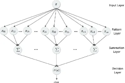
As shown in Figure 1, a PNN consists of four layers: the input layer, the pattern layer, the summation layer, and the decision layer. Among them, the input layer simply leaves the input data alone; the pattern layer receives the data from the input layer and calculates the probability that input data x equals the j-th layer neuron of the i-th layer of the pattern layer according to the defined kernel. The calculation formula can be expressed as Eq. (4):
T ij k 2 k 2 ( ) ( ) 1 ( ) (2π) σ 2σ ij ij x x x x x exp (4)
where Q is the number of training samples; R is the number of training samples in class i i 1, 2, 3, , Q)
( ; k is the dimension of the sample space data; σ is the smoothing factor; xij is the j-th j 1, 2,3,( , R) centre vector in class i.
Fig. 1 PNN structure
The summation layer adds up the output values of pattern layer neurons in the same class, and takes the average value of the output values. The calculation formula can be expressed as:
i N i ij i j 1 1 P ( ) ( ) N x x (5)The decision layer receives the output data from the summation layer, and estimates the maximum PNN class by the following formula:
i
class( )x arg max P ( )x (6)
The PNN is a powerful pattern classification method, including stable structure, short training time, high fault tolerance, good convergence and strong nonlinear recognition ability. The fundamental problem solved by Bayesian decision theory is to minimize the classification error rate, and the problem can be transformed into the estimation problem of solving the prior probability and the conditional probability. The prior probability expresses the proportion of the each type of sample in the sample space. According to the large number theorem, when the training set contains sufficient independent and identically distributed samples, the prior probability can estimate the frequency of occurrence of various samples. So, the method always produces the optimal solution by Bayesian criterion if there are sufficient training samples [38]. Despite these advantages, the PNN only applies to single-label pattern classification. Therefore, it was improved in the next sub-section into the IPNN to manage multi-label classification.
3.2 IPNN
(1) Multi-label PNN (ML-PNN)
In the multi-label classification, a label can be identified with two states: “0” or “1”. If an instance belongs to a label, the label value is “1”; otherwise, the value is “0”. When the traditional PNN is adopted for multi-label classification, the summation layer cannot sum up the output values. In order to solve the problem, the summation layer was replaced with the probability layer and the filter layer to manipulate multi-label data. Specifically, the filter layer saves lots of computing time by selecting part of the nearest neighbours to join the operation.
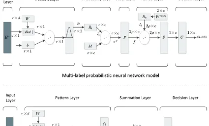
In addition, a revision layer was added so that the network can fully consider the label correlation. This new layer represents the label correlation and class information. Overall, the IPNN contains six layers: the input layer, the pattern layer, the probability layer, the filter layer, the revision layer and the decision layer.
Figure 2 compares the traditional PNN with the IPNN. It can be seen that the two models differ slightly in the input layer and the pattern layer. In Figure 2, H
h ,h ,h , ,h1 2 3 d
with H being the d-dimensional sample vector and hk being the k-th eigenvalue of the sample; W is the weight matrix and the number of pattern layer neurons; ||dist|| is the Euclidean distance between the input vector matrix H and the weight vector W; b is the vector matrix of network thresholds whose rows and columns are the same as d1; Wij is the j-th vector in class i; φij(H) is the kernel function of the similarity between H and Wij . If H is a training dataset, then W is the transposed matrix of the training data; If H is the test dataset, W is the transposed matrix of the test data.The pattern layer output can be calculated as:
* * T * ij ij ij d 2 d 2 ( ) ( * ) 1 φ ( ) ( 2π ) σ 2σ H W H W H exp (7)
where d is the dimension of the sample space data; σ is the smoothing factor. The input data and the weight matrix should be normalized before calculating the Euclidean distance, so that the features of the same instance have the same order of magnitude. Both H* and W*ij are the results of normalization, using Eq. (8). The Euclidean distance can be calculated as::
* min max min ( D V ) D (V V ) (8)
where D* is the normalized distance; D is the original distance; Vmin is the minimum; Vmax is the maximum.
In Figure 2, the rule R1 means converting matrix p1 to matrix l1,
l1
p1 p1 p1
.The dimension of l1 is c. M
M ,M ,M , ,M1 2 3 n
, Mi
m ,m ,m , ,mi1 i 2 i3 ic
, with M being the set of classes of all training samples, Mi being the multi-label class of the i-th instance,n being the number of classes for all training samples, being the dimension of the label,
and mij being the state value of the j-th label of class i (mij = 1 if the instance belongs to a
label and mij = -1 if otherwise).
Assuming that the c labels in class Mi are independent of each other and that only one pattern layer neuron Wi belongs to class Mi, then the parent probability or likelihood of H* belonging to class Mi can be expressed as:
* * T * * ij d 2 d 2 ( ) ( ) 1 φ ( ) ( 2π ) σ 2σ ij ij H W H W H exp (9)
Under these circumstances, the H* for the state value τi of class Mi can be calculated as:
i1 ii i2 i ic i
i φ ( ) m φ ( ) m φ ( ) m φ ( ) φ ( ) i i τ M H H H H M H (10)c
According to Eqs (7-10), it is possible to derive the similarities between H* and all pattern layer neurons and the state value matrix ( * )T
1 1 2 r
τ l M τ τ τ on all classes M,
where τj τj1 τj2 τjcT. As shown in Figure 2, τT is the output matrix of the probability layer.
In the filter layer, only valid data can join the subsequent network computation, aiming to prevent the inefficient computing and high memory usage under huge data size. The computing process can be expressed as:
j filter j j u τ δ (11) T 0,1 ρ r ,1 q ρ ρ 0 q j null 1j 2j ρj j u u u u u (12) T 0,1 ρ r ,1 q ρ ρ 0 q j null 1j 2j ρj j δ δ δ δ δ (13)
Through Eqs. (11), (12) and (13), all similar values of the j-th label in the state value matrix τ from the probability layer can be divided into positive and negative parts. The positive part, denoted as uj, contains the first ρ maximums, while the negative part, denoted as δj, contains the first ρ maximums of the absolute value.
Following the above rules, the filter layer uses the filter transfer function F to filter the state values of all the labels in matrix τ to obtain the output matrix τfilter. The positive part of τfilter is
denoted as u u1 u2 uc and the negative part as δ δ1 δ2 δc. Through the above steps, it is possible to identify the target label corresponding to the pattern layer neurons that are very similar to the target instance. In this way, the revision layer does not have to calculate all the probability values output of the probability layer. It only needs to calculate part of the value, and the interference from less similar target labels is eliminated. Eq. (10) is derived under the assumption that multiple labels are independent of each other. In actual practice, however, there is a correlation between the multiple labels. Considering this, the classification results were corrected by the weight matrix of the label correlation and the class information in the revision layer.
In the multi-label classification, the results are heavily influenced by the label correlation and the class information. Nevertheless, the two influencing factors have not been considered in most algorithms. To fully utilize the label correlation and the class information, a revision layer is introduced here with a weight matrix Wmulti. In the matrix,
the elements in each row stand for the weight information between the target labels, and the elements in each column refer to the weight information between classes. The value of the matrix is updated after each network training.
The Wmultiis a 2-row c-column vector matrix, in which the initial value of each element is 1:
1 2 c 1 2 c ψ ψ ψ 1 1 1 σ σ σ 1 1 1 multi W ψ σ (14)
where ψ and σ are the weight vectors of the positive part and negative part of τfilter, respectively; ψi and σi are the weight values of the i-th target label state values “1” and “-1”, respectively. The rule R2 represents a matrix l2 that extends Wmulti
to 2ρ×c: 1 2 c 1 2 c ψ ψ ψ 1 1 1 σ σ σ 1 1 1 multi W ψ σ (14) 2 ψ 2 σ 2 ψ ψ σ σ l l l (15)
where lψ2 and lσ2 are the members of a ρ×c matrix. The correction formula of the filter layer output matrix in the revision layer can be expressed as:
u δ s s s (16)
where s is the corrected state value matrix, i.e., the output matrix of the revision layer; su is the positive part of the corrected matrix; sδis the negative part of the corrected matrix. su and sδ can be expressed as Eqs. (17) and (18), respectively:
u u u u 1 2 ρ s s s s (17) δ δ δ δ s s1 s2 sρ (18)
Then, sρu and sρδ can be calculated as Eqs. (19) and (20), respectively: ψ u q q s = u (19) σ δ q ρ* s = u (20)
Based on the corrected state value matrix s f l 2, the probability of sample H falling into a label can be obtained by the summing transfer function S:
pro1 pro2 proc
pro (21)
The proj can be calculated as:
S 2ρ j yj y 1 pro
(22)The decision layer receives the pro vector, and obtains the multi-label class vector out through the competitive transfer function C:
out1 out2 outc
out (23)
The outi can be calculated as:
i i i 1 if pro 0 out 1 if pro 0 (24)
(2) Data-related learning
The weight matrix in the IPNN revision layer contains the information on the data correlation. Here, the IPNN was trained with the direction propagation mechanism, and the weight matrix of the revision layer was quantitatively updated according to the accuracy of the classification results. In Figure 2, matrices α and β stand for the positive and negative parts of the filter layer, respectively; W and W' represent the weight matrices of the positive and negative parts in the revision layer, respectively. Before network training, an error function was defined as follows. Let P be the probability vector of the final output of the IPNN. Then, this vector can be expressed as:
P1 P1 Pc
P (25)
where c is the number of labels in a class. By the definition, Pi represents the probability value of a label:
T T
i
P W α Ei( , ) W β Ei,( , ) (26)
where E is the row vector whose ρ elements are valued “1”; α' is the ρ-column row vector for the positive part of the i-th label; β' is the ρ-column row vector for the negative part of the i-th label.
Then, the value of P is normalized as:
P1 P2 Pc , P (27) ( ) i i P, T θ = p E (28) 1 2 c θ θ θ θ (29)
where P' is the matrix of the absolute values of all elements of P; ϑ is the normalized matrix of P; E is a c-dimensional row vector whose elements are valued “1”. Let R'' be the real classification vector corresponding to the input data x.
" "1 "1 "c
R R R R (30)
where c is the number of labels in a class. R'' only has two state values: “1” or “-1”. For the input data x, the error between the probability value and real value of the i-th label can be defined as: 2 1( ) , 1 i c 2 i E R" θ (31)
The result of the above equation is the error value of a label in the class. Thus, the error of the entire class Etotal can be obtained as:
total 1 2 c
E E E E (32)
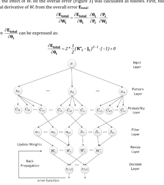
Next, the effect of Wi on the overall error (Figure 3) was calculated as follows. First, find the partial derivative of Wi from the overall error Etotal:
totali totali ii ii E E θ P W θ P W (33) where totali E
θ can be expressed as:
2 1 1 2* ( ) ( 1) 0 2 total i i i E R" J θ (34)
Fig. 3 IPNN structure
i i
θ
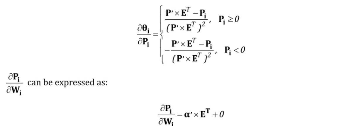
T T 2 T T 2 , 0 ( ) , 0 ( ) , i i , i , i i i , P E P P P E θ P P E P P P E (35) ii P
W can be expressed as:
0 , T i i P α E W (36)
The Eqs. (34), (35) and (36) can be calculated according to the known conditions. Therefore, the value of Eq. (33) can be obtained from these equations. Finally, the updated values of Wi can be obtained from
i i P W : η total i i i E W W W (37)
where η is the learning rate, i.e. the controllable speed of the learning process. The above steps form the computing process of the updated values of Wi. The values of other revision layer neurons can be updated in a similar way. The update of revision layer weights should be terminated after reaching the pre-set target error. At the termination condition, the weight of the revision layer can be applied to test the new input data.
4. NUMERICAL EXPERIMENTS
This section compares the proposed algorithm with several popular multi-label classification methods, namely CLR, BPMLL, RaKEL, Co-MLHN, ML-KNN, Multilabel ranking (MLR), Ensembles of classifier chains (ECC), and One-versus-all (OVA)-SVM.
4.1 DATASETS
Three public datasets from Mulan (http://mulan.sourceforge.net/datasets-mlc.html) were selected for the comparison, including Yeast, CAL500 and Emotions. The features of all multi-label data for our numerical experiments are listed in Table 1, where “multi-labels” is the number of labels in the dataset, “instances” is the number of instances in the dataset, “domain” is the type of data, “numeric” is the instance space, “cardinality” is the average number of positive labels per sample point.
Table 1 Information of Datasets
name domain instances numeric labels cardinality
CAL500 [39] music 502 68 174 26.044
Emotions [40] music 593 72 6 1.869
4.2 PARAMETER SETTING
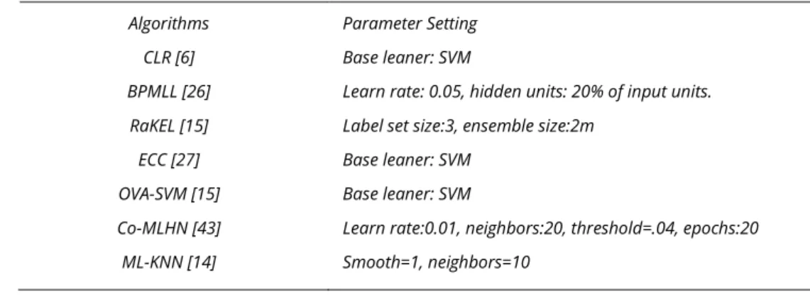
Table 2 introduces seven of the most popular multi-label classification methods. All the parameters were initialized with the recommended values of each algorithm [43]. For the ML-IPNN, the spread of the Gaussian function and the nearest neighbour range 𝜌were empirically obtained, the value of the learning rate for backpropagation in probabilistic neural network needs to be determined empirically. Currently, there is no effective way to automatically determine the learning rate. Therefore, this paper determines the optimal learning rate as 0.05. the target error was set to 0.01, and the number of iterations was set to 100 (http://mulan.sourceforge.net/download.html).
Table 2 Information of Datasets
Algorithms Parameter Setting
CLR [6] Base leaner: SVM
BPMLL [26] Learn rate: 0.05, hidden units: 20% of input units.
RaKEL [15] Label set size:3, ensemble size:2m
ECC [27] Base leaner: SVM
OVA-SVM [15] Base leaner: SVM
Co-MLHN [43] Learn rate:0.01, neighbors:20, threshold=.04, epochs:20
ML-KNN [14] Smooth=1, neighbors=10
4.3 EVALUATION METRICS
The classification results of all eight algorithms were evaluated against five metrics for multi-label performance, including the Hamming loss, example based f-1, one-error, ranking loss and average precision. Specifically, Hamming loss refers to the ratio of the number of inconsistent labels between the predicted result and the real result to the total number of labels [42]:
N i , j i 1 XOR(Y , ) 1 HamLoss N L i,j P (38)N is the number of samples, L is the number of labels, Yi , j is the true value of the j-th component of the i-th prediction result. Pi,jis the predicted value of the j-th component of the i-th prediction result.
Example based f-1 refers to the weighted harmonic average of accuracy and recall when the control accuracy and the relative classification effect of recall are 1:
Y Y M i i 1 i i i 1 2 h ( x ) 1 F M h ( x )
| | || || (39)One-error refers to the number of labels whose largest probability of prediction falls out of the real label set:
x
p y Y i i i 1 1 one error( f ) f , y Y p
arg max (40)Ranking loss is the number of times that the predicted probability of correlated labels is smaller than the predicted probability of uncorrelated labels through the comparison between the set of correlated labels and the set of uncorrected labels:
p s i i i 1 1 2 i 1 1 2 1 2 i i 1 L rlosss f p Y Y L ( y , y ) f x , y f ( x , y ), ( ( y , y ) ) Y Y
| | | || | | (41)Average precision examines the correct classification of labels in the sample's prediction label set prior to the sample label [43].
i i i i M i i f ( x , y ) i 1 y Y i i f ( x , y ) f ( x , y ) i a f 1 1 R ( x , y ) M Y r R ( x , y ) y r ) r e , y Y vepr (
| | | | { | } (42)The example based f-1 and average precision are positively correlated with the classification effect, while the remaining three metrics are negatively correlated with the classification effect.
4.4 COMPARISON RESULTS
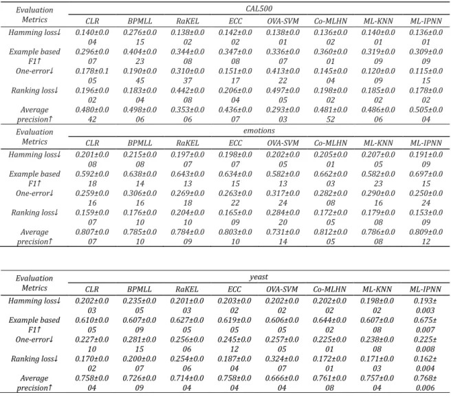
During the contrast experiment, there is no fixed ratio of the test samples and the training samples in the sample data. In this paper, 50% of each dataset was randomly extracted as the training data, and the remaining 50% was regarded as the test data. By this rule, 10 contrast experiments were conducted between the eight contrastive algorithms on each dataset. The datasets, algorithms, parameters, training data and test data are the same as those in Reference [43]. Thus, the experimental results on the three datasets were consistent with the results in Reference [43]. Then, the results of the ML-IPNN were contrasted with those of the seven algorithms against the five evaluation metrics (Table 3). In Table 3, ↑ means the metric value is positively correlated with the quality of the experimental result of an algorithm, while ↓ means the metric value is negatively correlated with the quality of the result.
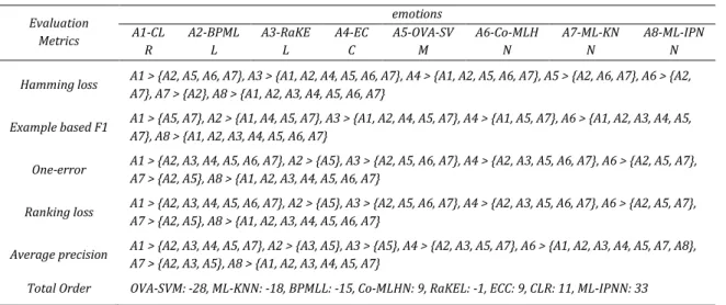
In order to evaluate the overall performance of each algorithm against all five metrics on each dataset, the classification results of any two algorithms were compared through a two-sample t-test at the significance level of 0.05 [14]. For any evaluation metric, if the results of algorithm A1 is better than those of algorithm A2, then the comparison result should be recorded as A1>A2, and algorithm A1 should acquire a positive score “+1”. On the contrary, algorithm A1 should
acquire a negative score “-1”. In this way, the score of each algorithm on each metric was obtained, and the total score of each algorithm on all five metrics were derived. Then, the algorithms were ranked by the total score, forming the relative classification effect of each algorithm on each dataset. If algorithm A1 achieves better effect than all the algorithms in the set l, the result should be recorded as A>{l}.
In the above tables, the “Total Ranking” shows the total score of each algorithm on each dataset. The algorithms are ranked in ascending order by the score [44].
Table 3 Multimeric comparison of the eight algorithms on three datasets
Evaluation Metrics
CAL500
CLR BPMLL RaKEL ECC OVA-SVM Co-MLHN ML-KNN ML-IPNN Hamming loss↓ 0.140±0.0 04 0.276±0.015 0.138±0.002 0.142±0.002 0.138±0.001 0.136±0.002 0.140±0.001 0.136±0.001 Example based F1↑ 0.296±0.007 0.404±0.023 0.344±0.008 0.347±0.008 0.336±0.007 0.360±0.001 0.319±0.009 0.309±0.009 One-error↓ 0.178±0.1 05 0.190±0.045 0.310±0.037 0.151±0.017 0.413±0.022 0.145±0.004 0.120±0.009 0.115±0.015 Ranking loss↓ 0.196±0.0 02 0.183±0.004 0.442±0.008 0.206±0.004 0.497±0.005 0.198±0.002 0.185±0.002 0.178±0.002 Average precision↑ 0.480±0.042 0.498±0.006 0.353±0.006 0.436±0.007 0.293±0.003 0.481±0.052 0.486±0.006 0.505±0.004 Evaluation Metrics emotions
CLR BPMLL RaKEL ECC OVA-SVM Co-MLHN ML-KNN ML-IPNN Hamming loss↓ 0.201±0.0 08 0.215±0.008 0.197±0.007 0.198±0.007 0.202±0.005 0.205±0.001 0.207±0.005 0.191±0.009 Example based F1↑ 0.592±0.018 0.638±0.014 0.643±0.013 0.634±0.015 0.582±0.013 0.662±0.003 0.582±0.023 0.697±0.015 One-error↓ 0.259±0.0 16 0.306±0.0 16 0.269±0.0 18 0.263±0.0 22 0.317±0.0 24 0.282±0.0 08 0.290±0.0 16 0.250±0.0 24 Ranking loss↓ 0.159±0.0 07 0.176±0.010 0.204±0.010 0.165±0.009 0.284±0.020 0.172±0.005 0.179±0.008 0.153±0.009 Average precision↑ 0.807±0.007 0.785±0.010 0.784±0.009 0.803±0.010 0.731±0.014 0.812±0.005 0.786±0.008 0.809±0.012 Evaluation Metrics yeast
CLR BPMLL RaKEL ECC OVA-SVM Co-MLHN ML-KNN ML-IPNN Hamming loss↓ 0.202±0.0 03 0.235±0.005 0.201±0.003 0.203±0.002 0.202±0.002 0.202±0.002 0.198±0.002 0.193± 0.003 Example based F1↑ 0.610±0.005 0.607±0.009 0.627±0.005 0.619±0.005 0.606±0.005 0.644±0.002 0.607±0.008 0.675± 0.007 One-error↓ 0.227±0.0 10 0.281±0.015 0.256±0.006 0.245±0.012 0.257±0.005 0.225±0.001 0.238±0.008 0.225± 0.008 Ranking loss↓ 0.170±0.0 02 0.200±0.007 0.254±0.006 0.187±0.004 0.324±0.007 0.172±0.001 0.171±0.003 0.162± 0.004 Average precision↑ 0.758±0.0 04 0.726±0.0 09 0.714±0.0 04 0.758±0.0 04 0.666±0.0 04 0.761±0.0 08 0.757±0.0 04 0.768± 0.006
Table 4 Relative classification effect of each algorithm on Yeast dataset
Evaluation Metrics
CAL500
A1-CLR A2-BPMLL A3-RaKEL A4-ECC A5-OVA-SVM A6-Co-MLHN A7-ML-KNN A8-ML-IPNN Hamming
loss
A1 > {A2, A4}, A3 > {A1, A2, A4, A7}, A4 > {A2}, A5 > {A1, A2, A4, A7}, A6 > {A1, A2, A3, A4, A5, A7}, A7 > {A2, A4}, A8 > {A1, A2, A3, A4, A5, A7}
Example based F1
A2 > {A1, A3, A4, A5, A6, A7, A8}, A3 > {A1, A5, A7, A8}, A4 > {A1, A3, A5, A7, A8}, A5 > {A1, A7, A8}, A6 > {A1, A3, A4, A5, A7, A8}, A7 > {A1, A8}, A8 > {A1}
One-error A1 > {A2, A3, A5}, A2 > {A3, A5}, A3 > {A5}, A4 > {A1, A2, A3, A5}, A6 > {A1, A2, A3, A4, A5}, A7 > {A1, A2, A3, A4, A5, A6}, A8 > {A1, A2, A3, A4, A5, A6, A7} Ranking loss A1 > {A3, A4, A5, A6}, A2 > {A1, A3, A4, A5, A6, A7}, A3 > {A5}, A4 > {A3, A5}, A6 > {A3, A4, A5}, A7 > {A1, A3, A4, A5, A6}, A8 > {A1, A2, A3, A4, A5, A6, A7}
Average
precision A1 > {A3, A4, A5}, A2 > {A1, A3, A4, A5, A6, A7}, A3 > {A5}, A4 > {A3, A5}, A6 > {A1, A3, A4, A5}, A7 > {A1, A3, A4, A5, A6}, A8 > {A1, A2, A3, A4, A5, A6, A7} Total Order OVA-SVM: -20, CLR: -10, RaKEL: -12, ECC: -7, ML-KNN: 6, BPMLL: 7, Co-MLHN: 14, ML-IPNN: 22
Table 5 Relative classification effect of each algorithm on CAL500 dataset Evaluation Metrics emotions A1-CL R A2-BPML L A3-RaKE L A4-EC C A5-OVA-SV M A6-Co-MLH N A7-ML-KN N A8-ML-IPN N Hamming loss A1 > {A2, A5, A6, A7}, A3 > {A1, A2, A4, A5, A6, A7}, A4 > {A1, A2, A5, A6, A7}, A5 > {A2, A6, A7}, A6 > {A2,
A7}, A7 > {A2}, A8 > {A1, A2, A3, A4, A5, A6, A7}
Example based F1 A1 > {A5, A7}, A2 > {A1, A4, A5, A7}, A3 > {A1, A2, A4, A5, A7}, A4 > {A1, A5, A7}, A6 > {A1, A2, A3, A4, A5, A7}, A8 > {A1, A2, A3, A4, A5, A6, A7}
One-error A1 > {A2, A3, A4, A5, A6, A7}, A2 > {A5}, A3 > {A2, A5, A6, A7}, A4 > {A2, A3, A5, A6, A7}, A6 > {A2, A5, A7}, A7 > {A2, A5}, A8 > {A1, A2, A3, A4, A5, A6, A7}
Ranking loss A1 > {A2, A3, A4, A5, A6, A7}, A2 > {A5}, A3 > {A2, A5, A6, A7}, A4 > {A2, A3, A5, A6, A7}, A6 > {A2, A5, A7}, A7 > {A2, A5}, A8 > {A1, A2, A3, A4, A5, A6, A7}
Average precision A1 > {A2, A3, A4, A5, A7}, A2 > {A3, A5}, A3 > {A5}, A4 > {A2, A3, A5, A7}, A6 > {A1, A2, A3, A4, A5, A7, A8}, A7 > {A2, A3, A5}, A8 > {A1, A2, A3, A4, A5, A7}
Total Order OVA-SVM: -28, ML-KNN: -18, BPMLL: -15, Co-MLHN: 9, RaKEL: -1, ECC: 9, CLR: 11, ML-IPNN: 33
Table 6 Relative classification effect of each algorithm on Emotions dataset
Evaluation Metrics yeast A1-CL R A2-BPML L A3-RaKE L A4-EC C A5-OVA-SV M A6-Co-MLH N A7-ML-KN N A8-ML-IPN N Hamming loss↓ A1 > {A2, A4}, A3 > {A1, A2, A4, A5, A6}, A4 > {A2}, A5 > {A2, A4}, A6 > {A2, A4}, A7 > {A1, A2, A3, A4, A5,
A6}, A8 > {A1, A2, A3, A4, A5, A6, A7} Example based
F1↑
A1 > {A2, A5, A7}, A2 > {A5}, A3 > {A1, A2, A4, A5, A7}, A4 > {A1, A2, A5, A7}, A6 > {A1, A2, A3, A4, A5, A7}, A7 > {A5}, A8 > {A1, A2, A3, A4, A5, A6, A7}
One-error↓ A1 > {A2, A3, A4, A5, A7}, A3 > {A2, A5}, A4 > {A2, A3, A5}, A5 > {A2}, A6 > {A1, A2, A3, A4, A5, A7}, A7 > {A2, A3, A4, A5}, A8 > {A1, A2, A3, A4, A5, A7}
Ranking loss↓ A1 > {A2, A3, A4, A5, A6, A7}, A2 > {A3, A5}, A3 > {A5}, A4 > {A2, A3, A5}, A6 > {A2, A3, A4, A5}, A7 > {A2, A3, A4, A5, A6}, A8 > {A1, A2, A3, A4, A5, A6, A7}
Average precision↑
A1 > {A2, A3, A5, A7}, A2 > {A3, A5}, A3 > {A5}, A4 > {A2, A3, A5, A7}, A6 > {A1, A2, A3, A4, A5, A7}, A7 > {A2, A3, A5}, A8 > {A1, A2, A3, A4, A5, A6, A7}
Total Order OVA-SVM: -27, BPMLL: -24, RaKEL: -7, ECC: -4, ML-KNN: 4, CLR: 8, Co-MLHN: 16, ML-IPNN: 34
Table 3 describes multiple scores for 8 algorithms on the three data sets. Table 4, Table 5 and Table 6 compare the scores of the eight algorithms on different evaluation indicators, and compare the sum of the scores of each algorithm on all evaluation indicators.
As shown in Table 4, on CAL500 dataset, the ML-IPNN had similar effect with Co-MLHN on Hamming loss, slightly outperformed CLR on the example based f-1, and outdid all contrastive algorithms on the other three metrics. In general, the ML-IPNN received the highest total score, followed by Co-MLHN. OVA-SVM once again ranked at the bottom.
As shown in Table 5, on Emotions dataset, the ML-IPNN was slightly worse than Co-MLHN on the average precision, but performed better than all the contrastive algorithms on the other four metrics. As for total score ranking, ML-IPNN came on the first place, CLR ranked second, Co-MLHN fell to the fifth, and OVA-SVM remained at the bottom.
As shown in Table 6, on Yeast dataset, the ML-IPNN shared the same effect with Co-MLHN on One-error, and outperformed all contrastive algorithms on the other four metrics. Overall, the
ML-IPNN achieved the highest total score, i.e. the best classification effect, following by Co-MLHN. The lowest score went to OVA-SVM.
According to the “Total Ranking” in the three tables, ML-IPNN scored the highest on all three datasets; Co-MLHN ranked the second on CAL500 and Yeast, and the fifth on Emotions; CLR occupied the seventh place on CAL500, the second on Emotions and third on Yeast; the other algorithms had different rankings on different datasets. It is sure to say that the ML-IPNN achieved the most stable classification effect.
Next, the performance of each algorithm on the three datasets was evaluated against each metric. The results are illustrated in Figures 4-8.
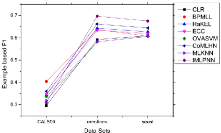
Fig. 4 The performance of the eight algorithms on example based f-1
Fig. 5 The performance of the eight algorithms on average precision
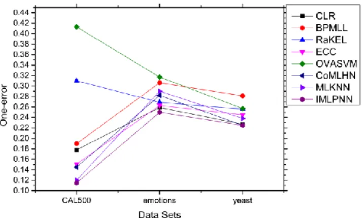
Fig. 7 The performance of the eight algorithms on one-error
Fig. 8 The performance of the eight algorithms on ranking loss
On the example based f-1, CLR, OVA-SVM and ML-KNN had the same effect on Yeast and Emotions. Their performance was poorer than the other algorithms. Among the remaining five algorithms, RaKEL, ECC and BPMLL performed worse than ML-IPNN and Co-MLHN. Specifically, the effect of ML-IPNN was better than that of Co-MLHN. On CAL500, ML-IPNN and Co-MLHN were outperformed by BPMLL. In summary, the example based f-1 shows that ML-IPNN performed better than the other algorithms on Yeast and Emotions, and slightly poorer on CAL500. The poor performance on CAL500 is attributed to the relatively high average positive label number per sample point in CAL500 (Table 1). In a word, the best performance was achieved by ML-IPNN.
On average precision, OVA-SVM and RaKEL respectively had the worst and second worst performance on all datasets. Meanwhile, BPMLL and ML-KNN had similar performance, but were both less efficient than Co-MLHN, CLR, ECC and ML-IPNN. ML-IPNN, and a little behind Co-MLHN in the performance on Emotions, but achieved the optimal effect on CAL500 and Yeast. In general, ML-IPNN was again the optimal algorithm.
On Hamming loss, ML-IPNN boasted better performance than all contrastive algorithms on all three datasets. The leading edge was not that obvious on CAL500, but significant on Yeast and Emotions. This is because CAL500 contains more labels than the other datasets. Despite its poor performance on example based f-1, ML-IPNN realized the top performance on Hamming loss.
On One-error, OVA-SVM and RaKEL did poorly on CAL500. Facing the relatively high average positive label number per sample point in the dataset, the two algorithms were unable to process the numerous classes that a single instance belongs to. ML-IPNN once again
outpreformed all contrastive algorithms on all datasets. Only ML-KNN had a comparable effect on CAL500. However, its effects on the other two datasets were far worse than that of ML-IPNN. Thus, ML-IPNN remained as the best performing algorithm on One-error.
On ranking loss, the eight algorithms performed similarly as they were on One-error. OVA-SVM and RaKEL had the poorest performance on all three datasets, while ML-IPNN still outperformed all contrastive algorithms on all datasets.
All in all, the ML-IPNN achieved better performance on each of the five-evaluation metric than the seven contrastive algorithms.
5. CONCLUSION
This paper presents a novel algorithm, the ML-IPNN, for multi-label classification. First, the traditional PNN was structurally converted into a neural network suitable for handling multi-label data. To improve the classification accuracy, a weight matrix was introduced to represent the label correlation and to synthetize the information between classes, and the ML-IPNN was trained with the backpropagation mechanism. Finally, the classification results of the ML-IPNN on three common datasets were compared with those of the seven most popular multi-label classification algorithms. The results show that the ML-IPNN outperformed all contrastive algorithms.
The future research should try to reduce the layer dimension and backpropagation mechanism of the algorithm without sacrificing accuracy and stability. Besides, the effect of ML-IPNN will be verified on large datasets and datasets containing numerous labels.
6. ACKNOWLEDGMENT
The research work was supported by National Natural Science Foundation of China under Grant No.61540050, Major Applied Basic Research Program of Guizhou Province under Grant No.JZ20142001, and Major Cooperation Science Research of Guizhou Province under Grant No.KH20173002.
7. REFERENCE
[1] S. Gao, W. Wu, C.H. Lee and T.S. Chua, A MFoM learning approach to robust multiclass multi-label text categorization, International Conference on Machine Learning, pp. 42, 2004., https://doi.org/10.1145/1015330.1015361
[2] J.Y. Jiang, S.C. Tsai, and S.J. Lee, FSKNN: Multi-label text categorization based on fuzzy similarity and k nearest neighbors, Expert Systems with Applications, Vol. 39, No. 3, pp. 2813-2821, 2012., https://doi.org/10.1016/j.eswa.2011.08.141
[3] F. Sun, J. Tang, H. Li, G.J. Qi and T. S. Huang, Multi-label image categorization with sparse factor representation, IEEE Transactions on Image Processing A Publication of the IEEE Signal Processing Society, Vol. 23, No. 3, pp. 1028-1037, 2014.,
[4] F. Briggs, B. Lakshminarayanan, L. Neal, X.Z. Fern, R. Raich, S.J.K. Hadley, A.S. Hadley and M.G. Betts, Acoustic classification of multiple simultaneous bird species: A multi-instance multi-label approach, Journal of the Acoustical Society of America, Vol. 131, No. 6, pp. 4640-4650, 2012., https://doi.org/10.1121/1.4707424
[5] K. Glinka, A. Wosiak and D. Zakrzewska, Improving Children Diagnostics by Efficient Multi-Label Classification Method, Springer International Publishing, pp. 253-266, 2016., https://doi.org/10.1007/978-3-319-39796-2_21
[6] G. Madjarov, D. Kocev, D. Gjorgjevikj and S. Deroski, An extensive experimental comparison of methods for multi-label learning, Pattern Recognition, Vol. 45, No. 9, pp. 3084-3104, 2012., https://doi.org/10.1016/j.patcog.2012.03.004
[7] G. Tsoumakas and I. Katakis, Multi-Label Classification: An Overview, I Int. J. Data Warehousing and Mining, Vol. 3, No. 3, pp.1-13, 2007.,
https://doi.org/10.4018/jdwm.2007070101
[8] M.L. Zhang and Z.H. Zhou, A Review on Multi-Label Learning Algorithms, IEEE Transactions on Knowledge & Data Engineering, Vol. 26, No. 8, pp. 1819-1837, 2014., https://doi.org/10.1109/TKDE.2013.39
[9] G. Dreyfus, Neural Networks: An Overview, pp. 1-83, 2005., https://doi.org/10.1007/3-540-28847-3_1
[10] W.B. Hudson, Introduction and overview of artificial neural networks in instrumentation and measurement applications, Instrumentation and Measurement Technology Conference, 1993. IMTC/93. Conference Record., IEEE, pp. 623-626, 1993.,
https://doi.org/10.1109/IMTC.1993.382568
[11] S. Godbole and S. Sarawagi, Discriminative Methods for Multi-Labeled Classification, Springer Berlin Heidelberg, pp. 22-30, 2004.,
https://doi.org/10.1007/978-3-540-24775-3_5
[12] L. Yi, J. Rong and Y. Liu, Semi-supervised Multi-Label Learning by Constrained Non-Negative Matrix Factorization, National Conference on Artificial Intelligence and the Eighteenth Innovative Applications of Artificial Intelligence Conference, July 16-20, Boston, Massachusetts, USA, pp. 421-426, 2006.
[13] M. Zhang, An Improved Multi-Label Lazy Learning Approach, Journal of Computer Research & Development, Vol. 49, No. 11, pp. 2271-2282, 2012.,
https://doi.org/10.1016/j.archoralbio.2005.12.006
[14] M.L. Zhang and Z.H. Zhou, ML-KNN: A lazy learning approach to multi-label learning, Pattern Recognition, Vol. 40, No. 7, pp. 2038-2048, 2007.,
https://doi.org/10.1016/j.patcog.2006.12.019
[15] G. Tsoumakas, I. Katakis and I. Vlahavas, Random k-Labelsets for Multilabel Classification, IEEE Transactions on Knowledge & Data Engineering, Vol. 23, No. 7, pp. 1079-1089, 2011., https://doi.org/10.1109/TKDE.2010.164
[16] R.E. Shaffer and S.L. Rose-Phersson, Improved probabilistic neural network algorithm for chemical sensor array pattern recognition, Anal. Chem. 1999, pp. 4263-4271, 1999., https://doi.org/10.1021/ac990238+
[17] X-Y. Sun et al., Improved probabilistic neural network PNN and its application to defect recognition in rock bolts, Int. J. Mach. Learn. & Cyber., 2016.,
[18] J-H. Yi, Improved probabilistic neural networks with self-adaptative strategies for transformer fault diagnosis problem, Advances in Mechanical Engineering, 2016., https://doi.org/10.1177/1687814015624832
[19] G. Kurata et al., Improved neural network-based multi-label classification with better initialization leveraging label co-occurrence, in proc. NAACL-HLT, San Diego, CA, USA, 2016., https://doi.org/10.18653/v1/N16-1063
[20] M.R. Boutell, J. Luo, X. Shen, et al. Learning multi-label scene classification[J]. Pattern recognition, 37(9): 1757-1771, 2004., https://doi.org/10.1016/j.patcog.2004.03.009
[21] D. Zhang, High-speed Train Control System Big Data Analysis Based on Fuzzy RDF Model and Uncertain Reasoning. International Journal of Computers, Communications & Control, 12(4), 2017., https://doi.org/10.15837/ijccc.2017.4.2914
[22] P.M. Ciarelli, E. Oliveira, C. Badue, et al. Multi-label text categorization using a probabilistic neural network[J]. International Journal of Computer Information Systems and Industrial Management Applications, 1(133-144): 40, 2009.
[23] J. Nam, J. Kim, E.L. Mencía, et al. Large-scale multi-label text classification-revisiting neural networks[C]//Joint european conference on machine learning and knowledge discovery in databases. Springer, Berlin, Heidelberg: 437-452, 2014.,
https://doi.org/10.1007/978-3-662-44851-9_28
[24] D. Montana, A weighted probabilistic neural network[C]//Advances in Neural Information Processing Systems, pp. 1110-1117, 1992.
[25] J. Fürnkranz, E. Hüllermeier, E. Loza, Mencía, & Brinker, K, Multilabel classification via calibrated label ranking, Machine Learning, Vol. 73, No. 2, pp. 133-153, 2008., https://doi.org/10.1007/s10994-008-5064-8
[26] M.L. Zhang and Z.H. Zhou, Multilabel Neural Networks with Applications to Functional Genomics and Text Categorization, IEEE Transactions on Knowledge & Data Engineering, Vol. 18, No. 10, pp. 1338-1351, 2006.,
https://doi.org/10.1109/TKDE.2006.162
[27] J. Read, B. Pfahringer, G. Holmes and E. Frank, Classifier Chains for Multi-Label Classification, Springer Berlin Heidelberg, pp. 254-269, 2009.,
https://doi.org/10.1007/978-3-642-04174-7_17
[28] M.L. Zhang, Ml-rbf: RBF Neural Networks for Multi-Label Learning, Kluwer Academic Publishers, pp. 61-74, 2009., https://doi.org/10.1007/s11063-009-9095-3
[29] Y.E. Kim, E.M. Schmidt, R. Migneco, B.G. Morton, P. Richardson, J. Scott, J.A. Speck and D. Turnbull, Music emotion recognition: A state of the art review, Proc. ISMIR, Vol. 86, No. 00, pp. 937-952, 2010.
[30] M.L. Zhang and K. Zhang, Multi-label learning by exploiting label dependency, ACM SIGKDD International Conference on Knowledge Discovery and Data Mining, pp. 999-1008, 2010., https://doi.org/10.1145/1835804.1835930
[31] G. Tsoumakas, I. Katakis and D. Taniar, Multi-Label Classification: An Overview, International Journal of Data Warehousing & Mining, Vol. 3, No. 3, pp. 1-13, 2007., https://doi.org/10.4018/jdwm.2007070101
[32] H.Y. Lo, S.D. Lin and H.M. Wang, Generalized k-Labelsets Ensemble for Multi-Label and Cost-Sensitive Classification, IEEE Transactions on Knowledge & Data Engineering, Vol. 26, No. 7, pp. 1679-1691, 2014., https://doi.org/10.1109/tkde.2013.112
[33] W. Bi and J.T. Kwok, Bayes-Optimal Hierarchical Multilabel Classification, IEEE Transactions on Knowledge & Data Engineering, Vol. 27, No. 11, pp. 2907-2918, 2015., https://doi.org/10.1109/TKDE.2015.2441707
[34] D.J.C. Mackay, Bayesian Methods for Neural Networks: Theory and Applications, Stat.purdue.edu, 1995.
[35] R.P.W. Duin, On the Choice of Smoothing Parameters for Parzen Estimators of Probability Density Functions, IEEE Transactions on Computers, Vol. C-25, No. 11, pp. 1175-1179, 1976., https://doi.org/10.1109/tc.1976.1674577
[36] E. Parzen, On Estimation of a Probability Density Function and Mode, Annals of Mathematical Statistics, Vol. 33, No. 3, pp. 1065-1076, 1962.,
https://doi.org/10.1214/aoms/1177704472
[37] M. Ahmadlou and H. Adeli, Enhanced probabilistic neural network with local decision circles: A robust classifier, IOS Press, pp. 197-210, 2010.,
https://doi.org/10.3233/ICA-2010-0345
[38] D.F. Specht, Probabilistic Neural Networks[J]. Neural Networks, 1990, 3(1):109-118., https://doi.org/10.1016/0893-6080(90)90049-Q
[39] D. Turnbull, L. Barrington, D. Torres and G. Lanckriet, Semantic Annotation and Retrieval of Music and Sound Effects, IEEE Transactions on Audio, Speech and Language Processing 16(2), pp. 467-476, 2008., https://doi.org/10.1109/tasl.2007.913750
[40] K. Trohidis, G. Tsoumakas, G. Kalliris and I. Vlahavas, "Multilabel Classification of Music into Emotions". Proc. 2008 International Conference on Music Information Retrieval (ISMIR 2008), pp. 325-330, Philadelphia, PA, USA, 2008.,
https://doi.org/10.1186/1687-4722-2011-426793
[41] A. Elisseeff and J. Weston, A kernel method for multi-labelled classification. In T.G. Dietterich, S. Becker and Z. Ghahramani, (eds), Advances in Neural Information Processing Systems 14, 2001.
[42] R.E. Schapire and Y. Singer, Boos Texter: A Boosting-based System for Text Categorization, Kluwer Academic Publishers, pp. 135-168, 2000.,
http://dx.doi.org/10.1023/A:1007649029923
[43] K.W. Sun, C.H. Lee and J. Wang, Multilabel Classification via Co-evolutionary Multilabel Hypernetwork, IEEE Transactions on Knowledge & Data Engineering, Vol. 28, No. 9, pp. 2438-2451, 2016., https://doi.org/10.1109/TKDE.2016.2566621
[44] H.K. Ghritlahre and R.K. Prasad, Investigation on heat transfer characteristics of roughened solar air heater using ANN technique, International Journal of Heat and Technology, Vol. 36, No. 1, pp. 102-110, 2018., https://doi.org/10.18280/ijht.360114